


Application / Solutions
Motor Design
Our accumulated knowledge and experience in motor design enables us to provide powerful yet easy to use simulation technologies.
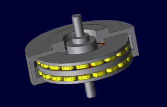
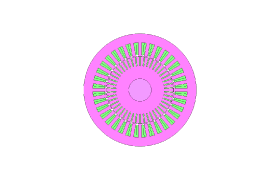
Axial Gap Type Motor
Axial-gap motors use an axial magnetic flux to rotate a disc-shaped rotor and stator facing each other.
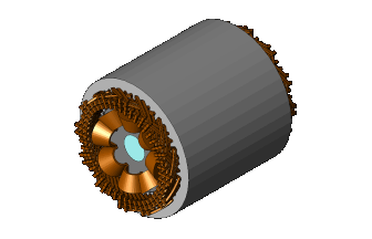
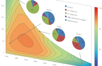
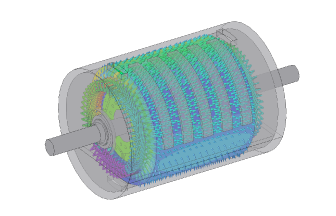
Wound Field Synchronous Motor
Wound-field and electrically-excited synchronous motors (WFSM/EESM) are given attention as traction motor that requires high efficiency in a wide operating range. Upd
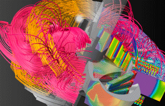
Induction Heating
JMAG correctly reproduces and visualizes the induction-heating phenomenon that changes intricately, and realizes the optimal design for various purposes using induction heating.
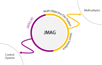
Model-Based Development
JMAG, which has a high track record in motor design, proposes a new workflow for model-based development.
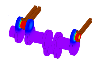
Thermal Analysis for Motor Design in JMAG
Within increasing demand for even higher efficiency and power in motor development, there is also the increase in demand for thermal design from electromagnetic design engineers. A thermal design method that balances both accuracy and ease of use is required in the electromagnetic design stage.

Utilizing JMAG in Cloud Services
Evaluating motor geometries and configurations at system design allows efficient development with less rework.
JMAG Open Interface programs
This page has been updated for ease of use and provides valuable information such as the necessity of coupled analysis, and the Multi-Purpose File Export Tool.
Case studies by users and applications for JMAG open interface programs are also available on this page. Upd
Case studies by users and applications for JMAG open interface programs are also available on this page. Upd