Overview

Axial gap motors can consist of a thinner construction than that of radial gap motors, and are used for in-vehicle motors where available space is otherwise limited. An optimal design is desired to maximize performance in this limited space.
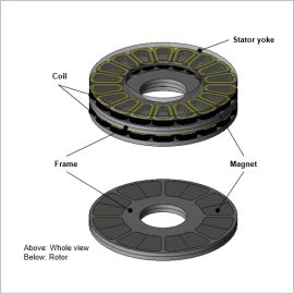
By running optimization calculations using Finite Element Analysis (FEA), globally optimal design proposals can be obtained from a wide design space. Because the magnetic flux that passes through the rotor and stator facing each other is a 3D magnetic circuit, the analysis model must be modeled as 3D geometry. Analyzing 3D geometry requires long calculation times. However, by using surrogate models, the amount of calculation time needed for optimization calculations can be reduced.
In this example, the dimensions of an axial gap motor are optimized by using surrogate models, then the Pareto curves and the effect of reduction in calculation times when using surrogate models are checked.

Optimization Conditions

The dimension variables and optimization conditions are shown in Fig. 1.
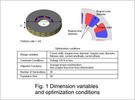
The design variables for the geometry dimensions are the frame width, magnet inner diameter, magnet outer diameter, and the flatness ratio.
The definition of the flatness ratio is height a/outer diameter b. The volume of the cylinder is assumed to be constant, and the height a and outer diameter b are uniquely determined by specifying the flatness ratio.

Using Surrogate Models for Optimization Calculations

The workflow of optimization calculations using surrogate models is shown in Fig. 2.
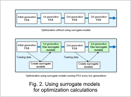
In optimization calculations using surrogate models, the calculation of particular generations is sped up by replacing surrogate models with machine learning models.
The training data is added to surrogate models after each FEA generation.

Pareto Curves

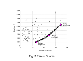
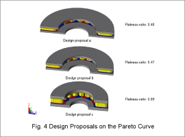
Fig. 3 shows the Pareto curves of the FEA intervals for every ten generations. Fig. 4 shows the designs obtained on the Pareto curves.
The Pareto curve uses up to 30 generations of data where optimization has converged.
It can be seen that the greater the torque, the smaller the flatness ratio and the flatter the axial gap motor geometry. This is because of the wider surface area of the gap where the torque generates. Conversely, the flatter the axial gap motor geometry, the smaller the cross section where the coils are wound, increasing the electrical resistivity. Copper loss increases, which results in an increase in total loss.

Effect of Reduction in Calculation Time When Using Surrogate Models

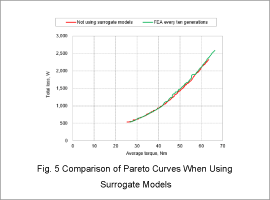
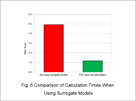
The Pareto curves both with and without using a surrogate model are shown in Fig. 5, and the calculation times are shown in Fig. 6.
Data up to 20 generations of converged optimization are used for comparison when the surrogate model is not used, and data up to 30 generations of converged optimization are used when the surrogate model is used.
Fig. 5 shows that the Pareto curve obtained using the surrogate model with the FEA intervals for every ten generations is equivalent to that obtained without using a surrogate model.
Fig. 6 shows that calculation times are reduced to 1/4 when the FEA intervals are for every ten generations.