What are FEA's Effects in the Development Process?
The purpose of this session is to show the merit of using simulation for the design of induction heating apparatus. Please consider the merits of analysis when you try to improve your heating method.
Overview
Induction heating is a kind of the electromagnetic induction phenomenon. When applying alternating magnetic field in a heating coil, eddy currents are produced in the surface of conductors. Its joule loss becomes the source of heat and the surface temperature rises. Induction heating apparatus span many fields, such as the induction hardening apparatus which improves the metallographic structure of the surface, the induction furnace which melts metal and is a meter in length. On the other side, there are medium-sized ones that warm up various liquids and solvents (Fig.1). The induction heating method has many merits, including local heating, rapid heating, high efficiency and direct heating by comparison with the combustion method.
It is difficult to get an optimized coil shape for various and complicated work pieces in a short time. Even though the geometry of a heating coil is defined, it is necessary to estimate the electrical power and frequencies for suitable depth of heating region from the surface. Spending a long time for heating, it results in heat conducting to the surrounding area and precise control of the heating process is not easy. In order to control increase in temperature while maintaining the objective heating range and depth, it is required to create many prototypes which change heating coils and power sources, or the intuition of experts would be another option.
The introduction of simulation causes a big change for the design of heating coils. Not only attempting the more suitable geometry and electrical power of the heating coil and power control and performing a reproductive experiment but also analyzing the process to such result of heating conditions, it allows you to obtain further improvements theoretically. Then you can get better design logically. We will show the simulation effects indicating the example of linear motor's bearing.
 Fig.1 Various applications
About analytical model
This model is the long square rod of carbon steel which has concaves on both sides. We try to treat induction hardening of the surface of the concaves. The concaves are bearing parts. To prevent it from becoming worn, we treat the surface treatment of concaves and increase hardness. If the depth of high temperature is large, the toughness of rod is lost. So, the target depth range to heat is a few millimeters from the surface. The observed points set three positions, the first one is the bottom of the concaves, the second is on the edge and the last one is the exterior surface (Fig.2). The alternating current was applied in heating coil, whose amplitude is 2000A, frequency is 30 kHz.
 Fig.2 Analytical model and observed points
Whether heating condition is satisfied?
Just preparing the geometry, setting the material, and setting the current or voltage on the heating coil makes it possible to create an analytical model. After completing an analysis, we can know the final temperature distribution and the heating time easily. If the heating time is long to some extent, we can control the current amplitude or the frequency. This model, which set the heating coil at 1.5mm away from the bottom, confirmed that the temperature of the bottom reach and over Curie points (about 700 deg C) after about 10 seconds (Fig.3).
 Fig.3 Temperature distribution after elapsing 10 seconds (left) Temperature transition (right)
Changing the position of Coil
If the position of heating coil is changed, the magnetic circuit is changed and the heating position and efficiency is changed. In this model, the coil position of 1.5mm has enough heating, but the position of 7mm is in lack of a heat source and temperature does not increase enough (Fig.4).
 Fig.4 Temperature distribution after elapsing 10 seconds(left : D=1.5mm, right : D=7mm)
Where do eddy currents flow?
Running an analysis makes it possible to indicate the locations where eddy currents flow in work pieces and the eddy current distribution offsets in the inner part of the heating coil as well. To raise the temperature of the surface, the eddy current must be generated in the target area. The distribution of eddy currents can investigate the validity of the position and shape of the heating coil and examine the next design. If D is 1.5mm, the large eddy currents are produced on the surface of the concaves (Fig.5 left). In order to heat only the surface of the concaves, it is better to place the heating coil closer so the amount of heat concentrated. On the other hand, when D is 7mm, the temperature rises on the outside surface as well (Fig.5 right). If we want to heat both inside of concaves and the outside, moving the heating coil further away is better. However, when setting it apart from the bottom, the heat generation amount is reduced. To make the surface treatment shallower, rapid heating is necessary and much more power source is required.
 Fig.5 Current density distribution at room temperature(left : D=1.5mm, right : D=7mm)
Checking the magnetic circuits
JMAG can indicate magnetic flux lines in 2D analysis and magnetic vector in 2D and 3D analyses. The eddy current flows to shield magnetic flux. Confirming the magnetic circuits is important to understand the induction heating process and the improvement of design. Please check where magnetic flux flows in test pieces. If D is 1.5mm, the magnetic flux flows from the heating coils to the surface of the concaves (Fig.6 left). This has the effect of concentrating the heat source on the bottom of the concaves. If D is 7mm, the magnetic flux flows from the heating coils to the outside surface (Fig.6 right). The eddy currents flow spreads widely an also enters from the bottom of the concaves and the exterior surface. The temperatures of the bottom rise simultaneously. If D is 7mm, the power is too little. The results of the case, whose amplitude of current is set at 3500A, are shown in figures 7 and 8. After heating for 10 seconds if we look at the temperature distribution shows, we can confirm that comparing with the position of D 1.5mm, the temperature rises both at the bottom and the outside (Fig.7). The temperature of the position of D 1.5mm rises rapidly on the bottom and the difference between the bottom and the surface is bigger, on the other hand, in the case the temperature of the position of D 7mm the difference between the surface of the concaves and the surface is smaller (Fig.8).
 Fig.6 Magnetic flux (left : D=1.5mm, right : D=7mm)
 (a) D=1.5mm,current 2000A (b) D=7mm, current 3500A
Fig.7 Temperature distribution after elapsing 10 seconds
 (a) D=1.5mm, current 2000A
 (b) D=7mm, current 3500A
Fig.8 Temperature transition of observed points
In Conclusion
The introduction of simulation can estimate the validity of design and can test a new idea easily. The distribution of each physical value inside work pieces shows new knowledge about the reason why this heating coil is better, then we can discuss logically about if there are more suitable designs. This text shows two dimensional section models, but JMAG supports complicated three dimensional models, off course. Please consider about induction heating analysis for your design.
(Hiroshi Hashimoto)
[JMAG Newsletter September, 2012]