Is FEA Effective in Motor Development?
This issue is aimed at those designing or using motors, to let you know the effectiveness of utilizing simulation. We hope you will find this useful as a reference for designing better motors.
Overview
This series has explained the issue of "Why is finite element method electromagnetic field analysis (hereafter FEA) effective in motor analysis?" Issue 1 discussed the use of FEA at the concept design and initial design stages for motors, and showed that use of FEA at the initial design stage allows high-speed investigation of design proposals with many degrees of freedom, which is difficult to calculate by hand. Issue 2 explained that, at the detailed design stage, FEA can be used for trial-and-error to economize on detailed designs. This final issue discusses the significance of FEA for detailed understanding of the phenomena that occur inside a motor.
Actual measurement tells you about performance and quality, but it does not tell you what the issues are
Prototypes are produced in order to evaluate whether developed products that have passed through concept design and detailed design can display performance as expected from their design, and their performance is measured using measuring devices or test benches. For example, the quality of a design can be evaluated by using measurement with a motor test bench to see if its output is as intended. These results come out clear and in black and white, but do not tell you the reason why the desired performance was not achieved, or what needs to be improved (fig. 1). Hints can be found through careful analysis of measurement results, but there are many design elements (causal elements), so it is not easy to find the cause.
 Fig. 1 Actual measurement can tell you about quality and provide hints, but...
Measurement is not easy
Measurement itself is not easy. For example, reduced loss and improved efficiency are constant goals for motors, and ever more reductions in loss are desirable in development. However, motors have become more efficient compared to earlier times, with amounts of loss that are normal today representing a large part of the work to be done, so more attention is being paid to areas where loss reduction can only be achieved by very close examination. It is as though most of a great feast has been finished, and it is now a matter of scraping up what is left around the edges.
Let's take iron loss measurement as an example. In theory, iron loss is separated into hysteresis loss and eddy current loss, but these cannot directly be measured separately, so they are separated by using theoretical formulas on measurement results. Traditionally, measurements using Epstein's method have been used to measure the loss in a laminated core. JMAG's iron loss tool also obtains iron loss using this data during practical calculation, and this method is thought to provide a certain degree of accuracy even now.
However, with reductions in motor size, operation in high frequency and high magnetic flux density regions that were not used previously is increasing in order to promote higher performance, and iron loss in these operation regions is getting more attention. Superimposed direct current has a large effect on loss in these regions, but Epstein's method is not adequate for loss measurement with high frequency and high magnetic flux density because it cannot account for superimposed direct current. Because of this, analysis using these results does not have sufficient accuracy, so something needs to be done to improve accuracy. Further, measurement itself is becoming more difficult because high-output and high-fidelity power supplies are necessary to measure loss with high frequency and high magnetic flux density (fig. 2).
 Fig. 2 Loss measurement of a ring core
Using FEA to bolster understanding and analysis of real phenomena
This is where FEA shows its effectiveness. FEA theoretically allows complex phenomena to be analyzed by modeling various physical phenomena. In reality, it is extremely difficult to "model all physical phenomena," but modeling with attention to the physical phenomena that are thought to make large contributions and the phenomena that are being focused on makes it possible to estimate how much influence these have.
Returning to the example given above, in order to find iron loss, which is difficult to measure, faithfully modeling material behavior and running analysis, such as using FEA to trace materials' hysteresis loops or directly analyze eddy current behavior, can be a great help in confirming and understanding their behavior. By comparing these analysis results with measurement results and interpolating them with each other, phenomena that could not previously be understood can now be understood, which should provide hints as to what can be done in response to the problem (fig. 3).
 Fig. 3 Analysis results can help in factor analysis
If evaluation of all physical phenomena is done in advance and development is carried out ideally exactly as designed, problems should not be discovered at the prototype evaluation stage, but sometimes events occur that are unexpected and whose cause it is difficult to know. In these situations, the correct approach is to compare measurement results with expectations from analysis, make use of all available information, and find a way to learn the cause and create a response plan.
JMAG loss analysis functions to improve model fidelity in line with theory, in order to come closer to real phenomena
In order to realize "FEA for understanding detailed phenomena," this section introduces the recently released JMAG-Designer's new functions for improving material loss analysis accuracy for laminated steel sheet.
Material properties modeling and iron loss eddy current components
In order to accurately analyze eddy currents in laminated steel sheet using FEA, ideally one would model the steel sheets one by one before analysis. However, this is not practical because it would mean an enormous calculation scale in reality. The function that solves this problem with practical calculation is "Eddy Current Loss Calculation for Laminated Steel Sheet." This analysis function itself was released in JMAG-Designer Ver.12.0, so many readers are probably already aware of it, but I would like to introduce it once again.
This function one-dimensionally obtains eddy currents (skin currents) in the lamination direction of laminated steel sheet from time variations in the magnetic flux density and the material's permeability, electric conductivity, and lamination thickness, making it possible to obtain eddy current loss from 2D analysis results. For 2D analysis, the concept is like 2D + 1D (fig. 4).
 Fig. 4 Concept of modeling in Eddy Current Loss Calculation for Laminated Steel Sheet
This method makes it possible to reduce calculation time to a manageable amount of time because it does not generate mesh in the lamination direction. It can also be applied to 3D analysis models. It has the disadvantages that in reality it ignores existing currents that are turned back in the lamination direction and that it is necessary to make a distinction with in-plane eddy currents, but it makes it possible to estimate the eddy current component of the iron loss in transient analysis, which was not possible with earlier iron loss analysis tools.
One of the problems raised in measurement (Epstein's method) is that high frequency and high magnetic flux density measurement is very difficult. As mentioned earlier, a high-quality, large-current power supply at high frequency is needed to carry out measurements in these regions. However, because it is difficult to get this kind of power supply, high-frequency loss outside the measurement range is obtained using extrapolation from low-frequency measurement results as a quadratic function of the frequency. Because of this, the higher the frequency is, the stronger the tendency toward overestimation, which causes error to be produced.
Eddy current loss can be obtained with high precision using the Eddy Current Loss Calculation for Laminated Steel Sheet function because eddy current loss is solved almost directly, making extrapolation unnecessary, and because it is possible to account for the phenomenon of the skin depth becoming thinner with increasing frequency. Loss can be understood with precision by comparing this function and measurement results, helping to solve the problem.
Material properties modeling and iron loss hysteresis components
I will introduce functions for improving analysis accuracy for hysteresis loss here, like I have for eddy currents. The policy for modeling the phenomena is, of course, to try to grasp hysteresis precisely.
Recently, motors with PWM drive have increased, but with PWM drive, the current waveform supplied to the motor has time harmonics superimposed by switching in addition to the fundamental wave. Accordingly, when seen on a micro level, its shape oscillates due to time harmonics in areas with DC offset caused by the fundamental wave. Because of this, the operating state of the magnetic circuit also has circulating minor hysteresis loops caused by superimposed DC.
Measurements made with Epstein's method cannot evaluate the effects of superimposed direct current because they measure loss by adding an alternating magnetic field around the zero point. The effect is small even with offset from superimposed DC so long as the operating state has relatively low saturation, but hysteresis loops become dramatically larger when saturation regions of silicon steel sheet are used (fig. 5). This means that the hysteresis loss is different for cases with and without superimposed DC.
 Fig. 5 Hysteresis loss
Recently, operating magnetic flux densities have been made higher in order to advance the miniaturization of electric motors, and it is often thought that a certain amount of magnetic saturation is inevitable so that, combined with the effects of PWM drive, the danger of hysteresis loss becoming larger than expected has become greater.
Functions have been implemented as of JMAG-Designer Ver.12.1 for carrying out magnetic field analysis accounting for hysteresis minor loops. Previously this was done using user subroutines, but it can now be set from the user interface. Regarding the issue of creating materials' hysteresis loops, a function is available, only for silicon steel sheet with iron loss properties, for automatic creation of hysteresis loops using that material's data. This is in addition to the method of users defining their own loops as point sequences.
Geometry modeling and magnet eddy current loss evaluation
Magnet temperature issues due to eddy current loss in magnets and reduced performance that comes with them are big problems for permanent magnet motors. The magnets are often incorporated into the rotor, so it is technically difficult to take temperature measurements of loss occurring in the magnetic substance while it is rotating.
In order to estimate this loss using analysis, it would be ideal to run a 3D analysis and an analysis with simulation of the eddy currents flowing in the magnets, but this is not practical because the calculation scale of 3D analysis is too large. As I explained in Issue 2, by using 2D analysis results and 3D analysis of the rotor only with magnetic flux boundary conditions applied, it is possible to calculate loss in the magnets with high precision in a reasonable calculation time (fig. 6).
 Fig. 6 Heat generation distribution
Functions for geometry modeling and stray load loss calculation
Like magnet eddy current loss, stray load loss is another area where some overlooked tidbits may be picked up. For example, eddy current loss produced in a motor case by leakage flux and coil ends is one possibility. These losses are relatively small, and measuring them individually is very difficult.
For this reason, it is important to confirm in advance that they are quantitatively small by calculating the losses using analysis. When loss is found to be larger than design values after the fact, a check must be done to see whether stray load loss is being produced in unexpected places.
Stray load loss is produced in motor cases, etc., so it is necessary for analysis to model all of the parts from which the motor is constructed, which requires 3D analysis. JMAG includes the following three functions to support the pursuit of stray load loss while both preserving calculation accuracy and controlling calculation scale in 3D analysis.
- Extended slide mesh
- Extruded mesh
- Coil end creation functions
With extended slide mesh functions, it is now possible to use slide mesh in geometries in which the motor cover is overhanging, which was not possible with previous cylindrical meshes. This makes it possible to obtain eddy currents with a higher degree of stability than when using patch mesh (fig. 6).
When extruded mesh is used to confirm a geometry such as a motor that has an identical cross-section at any point along its length, it uses 2D and extrusion to make a 3D mesh for that part, so the number of divisions in the radial and axial directions can be set appropriately. This allows a 3D model to preserve calculation accuracy while avoiding increases in the number of elements (fig. 7).
Fig. 7 Combination of expanded slide mesh and extruded mesh
Coil end creation functions allow the simple creation of coil end solids that are difficult to create as geometries in CAD. In order to consider stray load loss, the effects of the magnetic field created by the coil ends must be evaluated, so modeling functions are necessary for the coil ends (fig. 8).
 Fig. 8 Geometry created using a coil end template
These analysis functions make it easy to evaluate stray load loss.
Ways to increase calculation speed for detailed analysis
It is unavoidable that the scale of calculations for these high-precision calculations will grow large. For this reason, solvers that can process large-scale models with high speed are indispensable. In addition to a reevaluation of calculation methods, efforts have been made to extract better performance from hardware in order to achieve higher solver speeds in JMAG. It is well known that SMP and DMP are now common ways of increasing calculation speed with parallel processing by multiple CPUs or cores, but it is now also possible to use GPUs (Graphic Processing Units) intended for image processing to accelerate calculation.
These developments in modeling and calculation technologies have increased analysis precision, so analysis of measurement data is more powerfully supported.
Detailed analysis functions other than for loss
I have mainly focused here on functions for accurate loss calculation, but JMAG can also be used for detailed calculations other than for loss. For example, development is ongoing for consideration of degradation of magnetic properties due to stress by combination with structural analysis, and simpler linking with other applications for thermal fluid analysis, making it easier to do investigations that straddle multiple physical domains.
In Conclusion
Over these three issues, I have explained the effectiveness of FEA in motor development. JMAG is constantly striving for improved functionality and increased performance, but we will never be able to completely keep up with our users' ever-increasing demands. Still, we are continuing with our development so that we will not be left too far behind, and it is our greatest wish to provide a tool that will be even a little useful for all of you.
(Yoshiyuki Sakashita)
[JMAG Newsletter July, 2013]