Contents
- Copper Loss Analysis of a Rotating Machine
- Zooming Method Procedure and Overview
- Applying the Zooming Method to Rotating Machine Copper Loss
3.1 Copper Loss Characteristics Analysis of a 2D IPM Rotating Machine
3.2 Loss Analysis of Litz Wires in a Rotation Machine - Conclusion
- References
1. Copper Loss Analysis of a Rotating Machine
There is an electromagnetic field analysis using the finite element method (FEM) as an effective analysis method for copper loss accounted for eddy currents in the winding of a rotating machine. Although calculation accuracy can be achieved with this method, there are disadvantages such as requiring wires to be modeled one at a time, which increases the number of elements and increases calculation time by an enormous amount.
The zooming method (1) serves as a method to reduce these types of generic calculation cost issues. This method first solves a coarse mesh for the entire area (whole analysis), inherits those results, models in detail only a single section to obtain detail in, and then performs a partial analysis. This allows the number of elements of each complete/partial analysis to be reduced, improves convergence, and shortens calculation times.
As preceding examples, reference (2) proposes a magnetic flux density distribution and references (3) and (4) propose vector potential on a boundary to be inherited from a whole analysis to a partial analysis, and successful results were obtained for each proposal.
However, the calculation time and accuracy of the analysis using the zooming method for rotating machines have not been sufficiently evaluated. In this paper, this method is applied to a copper loss characteristics analysis of wires in a 2D rotating machine as well as a loss analysis of litz wires in a 3D rotating machine, and then an evaluation is performed for improving calculation accuracy and calculation speed. Unless otherwise indicated, this paper will hereafter refer to the method of inheriting vector potential on the boundary as the "zooming method".
2. Zooming Method Procedure and Overview
First, a whole analysis is performed, and all vector potential values of the time history to be calculated are obtained. Next, detailed mesh for the section to obtain accuracy is generated while simultaneously performing a calculation that inherits the information of the area calculated in a whole analysis. This inheritance uses vector potential components in the tangential direction on the model boundary for each time history. When internal forced current, permeability, and electric conductivity distribution are identical in the whole analysis and partial analysis, it is guaranteed that internal magnetic flux density B and eddy current density Je distribution will be identical (5).
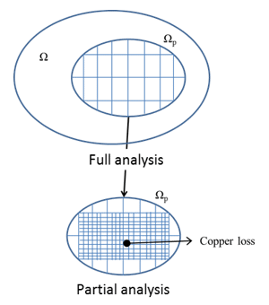
Fig. 1 Zooming method concept
3. Applying the Zooming Method to Rotating Machine Copper Loss
3.1 Copper Loss Characteristics Analysis of a 2D IPM Rotating Machine
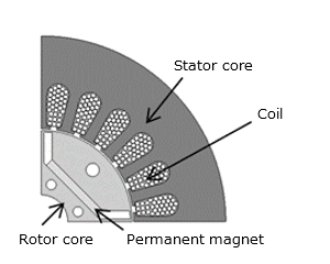
This section displays a use case in which the zooming method is used on a copper loss characteristics analysis of a 2D IPM rotating machine. The analysis target is set as The Institute of Electrical Engineers of Japan (IEEJ) D model (6), the zooming method is applied to the copper loss characteristics calculation for each rotation speed, and the calculation accuracy and calculation speed are evaluated.
Condition details of the motor under evaluation are shown in Table 1. For the analysis time interval, electric angle period is divided into 192. Input is set to current, and the waveform has the same amplitude regardless of the rotation speed, and only differs by frequency. The analysis region is set as 1/4 symmetry model. These are common conditions, regardless of whether the zooming method is used.
Table 1 Model details
| Number of Poles | 4 |
|---|---|
| Number of Slots | 24 |
| Wire Diameter, mm | 0.65 |
| Number of Turns/Phase | 140 |
| Current Amplitude, Arms | 3 |
| Number of Phase | 3 |
| Rotation Speed, rpm | 500, 1500, 3000, 5000, 7000, 10000 |
An analysis model not using the zooming method is shown in Fig. 2. As shown in Fig. 2 (a), each wire is modeled individually, and the mesh in the wire is finely divided as in Fig. 2 (b).
(a) Analysis model
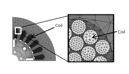
(b) Finite element mesh (without air region)
Fig. 2 Analysis model when not using the zooming method
You need to sign in as a Regular JMAG Software User (paid user) or JMAG WEB MEMBER (free membership).
By registering as a JMAG WEB MEMBER, you can browse technical materials and other member-only contents for free.
If you are not registered, click the “Create an Account” button.
Create an Account Sign in