Fig. 1

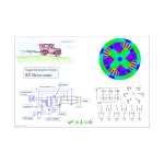
Video 54 introduced a short series of three or four videos with an attempt to compare flux-linkage captured at the terminals of an electric machine with oil captured at the well-head in an oil-field. It also likened our activities with the finite-element method to Goethe’s Sorcerer’s Apprentice,¹ who lost control of a water process just as we might sometimes lose control of a finite-element process. The common idea in these analogies is that oil, water, and flux are all useful and (at least for now) plentiful substances; but they need to be harvested or collected in a way that makes it possible to control and use them effectively and efficiently.

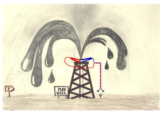
In electromagnetic analysis I like to think of myself not as the Sorcerer’s apprentice, but as Maxwell’s apprentice. It is not far from here to Maxwell’s birthplace and family home in south-west Scotland (Engineer’s Diary No. 58), and by an extraordinary coincidence it is also not far to the Five Sisters oil bings near Edinburgh, ^2,3 where the oil industry originated at almost the same time as the publication of Maxwell’s equations in the mid-19^th century. (It is also not far to the home of James Watt in Greenock, and the Carron Iron Works where cast iron parts were manufactured for his steam engines, a hundred years earlier). ⁴

For readers who enjoy history, there is plenty of it in the foundations of our modern world of numerical analysis and advanced manufacturing and materials. But let’s focus on the particular story that starts in Video 54. It is a very narrow, specific example of the productive use of finite-element data to generate practical engineering results, in the context of the inverter-fed synchronous machine (particularly the brushless AC PM machine). The F.E. data comes in the form of a record of phase flux-linkage and phase current through one electrical cycle. A little bit like the Sorcerer’s apprentice, we generate dozens of practical engineering results, one after the other; but unlike the uncontrollable pails of water, these results are limited in number and quite specific in their application, so perhaps it is more comfortable to think of ourselves as Maxwell’s apprentice, not the Sorcerer’s apprentice. We must also be careful to interpret and use the results correctly, because we cannot expect the Sorcerer to return and restore order; in that sense, we are alone!

Think of flux as oil gushing from a well. ⁵ Think of flux-linkage as oil captured at the well-head. The well-head is analogous to the terminals of an electric machine. Think of the finite-element method as a vast underground reservoir of unlimited quantities of flux. We don’t simply allow it to gush. We capture it at the terminals to derive a wide range of practical engineering results, just as oil is used to derive a wide range of useful chemicals and products. Using Faraday’s law, we can use flux-linkage immediately in the circuit analysis of the machine and the design of its controller. This applies not only to the ordinary flux-linkages, voltages, and currents of the actual phases or windings, but also to the transformed flux-linkages, voltages, and currents found in dq axes or αβ axes.

We might take this for granted. But in fact the range of useful practical results is quite extraordinary, and the series beginning in Video 54 describes a systematic process in which many of them are obtained from a simple standard finite-element calculation. Here we will define the finite-element calculation and summarise some of the main results as they relate to the common example of a brushless permanent-magnet machine.

It’s important to start with the observation that the finite-element method by itself does not produce RMS values of AC quantities directly. It does not produce a peak value without a searching process to find the peak. It does not produce harmonics without Fourier series (for periodic functions) or the Fourier transform (for transients). It works only with real windings, and not directly with transformed equivalent windings such as those we use in dq axes. In connection with all these cases, it is therefore necessary to rotate the rotor and extract the required waveforms in the form of a sampled-data record covering one electrical cycle.

It is then necessary, as a further step, to perform additional processing to extract the parameters of interest. We often see a rich selection of general ‘post-processing’ functions bundled with the finite-element software; but this post-processing may not be formulated to provided everything the specialist user needs. It will generally be formulated and presented in the style (and with the conventions and nomenclature) of the finite-element software, which may be different from the user’s own.

It follows from all this, as we’ve suggested, that the essential finite-element calculation should be to rotate the rotor in steps through one electrical cycle, usually with sinewave currents fed to the phase windings. The amplitude and phase of these currents are defined by the controller at any operating point. The essential finite-element data is a record of the phase flux-linkage as a function of the rotor position, and synchronous with the applied current waveform. By ‘essential’ we mean that this data cannot be computed accurately by any other method. Let’s call this record yU. For the purposes of this article, let’s assume balanced conditions so that we need consider only one phases. (The process is still valid for unbalanced operation).

In the first instance we will be interested in the mean electromagnetic torque and the AC voltage required to drive the applied current. Both of these can be computed from the flux-linkage and current waveform records without further finite-element analysis. This is an important point because such post-processing can be done almost instantaneously once the necessary finite-element data is available. The same applies to many other processed results, as discussed below. The flux-linkage and current waveforms over one cycle permit detailed analysis of the instantaneous torque and the harmonics in the form of several other waveforms including not only the torque but also the dq components of flux-linkage and inductance. These are important in relation to torque ripple and control stability.

The ‘excited’ finite-element solution is in fact sufficient to calculate everything we need to know about a single operating point, at least in terms of terminal quantities. But engineers often want to know the generated EMF as well. The EMF is observable only on open-circuit, which is really a separate operating point requiring a second finite-element calculation with zero current.  It is generally straightforward to script the finite-element program to perform the two finite-element solutions concurrently or in sequence, or even to do several calculations covering a range of operating points. We do not need to go into detail on that aspect, but it will be helpful to identify the flux-linkage waveform of phase U as yU in the ‘excited’ solution, as already mentioned, and yU0 in the ‘open-circuit’ solution. These waveforms contain all the data that we need for our engineering calculations.

So: given yU and yU0, what can we do with them?

The first obvious thing to do is to display them — usually yU, yV, yW above or below the current waveforms iU, iV, and iW with which they are synchronous (but not generally in phase). While this is a simple task, it is a satisfying one because it shows the finite-element data directly as though we were looking at an oscilloscope. For many practical engineers this may be a more comfortable ‘view’ than a finite-element flux-plot or even a phasor diagram. For many decades these waveforms could not even be calculated, much less displayed: only their idealised forms (drawn by hand) were available in textbooks.

At this point the results can be scaled according to a change in the number of turns in the windings: for example, doubling the turns will double the flux-linkage waveforms exactly, while it halves the current for the same operating point. Similar arguments apply to changes in the number of parallel paths in the winding. Note that the winding factors do not arise anywhere in these processes, because we are dealing with the raw physics of coils of wire and Faraday’s law; the winding factors are ‘highly derived’ parameters that characterize the winding distribution in terms of ideal flux-density distributions (that cannot be realised in a finite-element solution!) If the finite-element solution is 2D, the flux-linkage waveforms can also be scaled according to the stack length and/or the stacking factor of the laminations, while the current waveforms remain unchanged. These scaling principles help to improve the utilization of the slower (but vital) finite-element process, which need not be repeated while we search for the right number of turns or adjust the stack length. They can also be used by design engineers who have no access to the finite-element process, or no skill in using it, or no free time!

The next natural operation might be to differentiate the yU0 waveform to get the generated open-circuit EMF. This involves differencing successive samples in the flux-linkage record, and scaling according to the speed. This itself is a handy feature, in that the EMF can be scaled exactly in proportion to the speed, just as it goes linearly with the turns. The finite-element solution is independent of speed and would often be a magnetostatic solution (though this is not a necessary requirement).

The EMF waveform will be that of one phase of the winding. Under balanced conditions the EMF waveforms of the other phases can be obtained by phase-shifting. Once we have them we can obtain the line-line waveform (the one that is normally measured) by subtracting the EMF waveforms of two adjacent phases. From this data we can quickly calculate the peak, RMS, and rectified mean values of both the phase and the line-line EMF waveforms.

It is often required to determine the main harmonics in the EMF waveform, using Fourier series (not the FFT).  It is also becoming common to require the THD (total harmonic distortion). Strictly speaking, the THD requires the calculation of an infinite number of harmonics, but this is clearly not practical since it would require unrealistic mesh densities and infinitesimally small rotor position steps. A decision must be made to limit the number of harmonics in the THD calculation, and this decision must take note of the sampling interval in the EMF waveform to avoid aliasing and the appearance of spurious (and non-existent) harmonics.

Under balanced conditions the harmonic analysis of the phase EMF waveform is sufficient also for the line-line EMF waveform. If the winding is connected in star this means dropping the triple-n harmonics (and scaling all the others by √3; but for delta connection there is no difference).

Up to this point we might think there is nothing new or exciting in this process; after all, it has been practised with the finite-element method for at least 40 years and maybe more. For sinewave synchronous machines, further analysis is almost always performed in dq axes, especially for steady-state operation, and this is where it becomes a little more interesting. 

In dq axes the steady-state is one in which, ideally, all voltages, currents, and flux-linkages are constant. But this does not have to be assumed a priori. When we have the three flux-linkage waveforms and the three current waveforms, we can transform them into dq components using Park’s transform, regardless of their actual waveshapes. With sinewave currents the dq components of current will be constant; but the flux-linkage waveforms will generally not be constant. There will often be a ripple component containing (typically) 6^th and 12^th harmonic components. If we calculate the torque using the equation

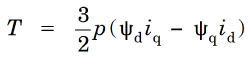(1)

it will have a 6^th and maybe a 12^th harmonic ripple; and if we calculate the synchronous inductances using the equations

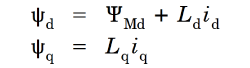(2)

they will also have a 6^th and maybe a 12^th harmonic ripple. We are looking at time-waveforms in dq-axes, which may seem strange since the dq transformation was surely devised to get away from time waveforms and view the machine operation in an ideal steady state, in a frame of reference fixed to the rotor, in which all quantities are constant. But we find that the quantities we thought fixed may actually be varying cyclically at a harmonic frequency. What a nuisance! But it is a practical fact.

The obvious component of interest is the torque, because torque ripple is always a matter of concern (independently of cogging torque, which arises from a different source). But variation in the synchronous inductances with rotor position is not often mentioned. It may be important in certain field-oriented controllers that are designed on the assumption that this ripple does not exist.

Note that this data — the waveforms of current, flux-linkage, and torque — in dq axes comes effortlessly from the same essential finite-element calculation mentioned at the start. It requires no additional finite-element analysis, because the necessary data is already inherent in the waveform data.

Many more interesting waveforms, parameters, and diagrams can be deduced easily from the same waveform data. For example, the Lissajous figure of the Clarke components of EMF shows immediately the presence of any harmonics (although it does not give their amplitudes). The Lissajous figure of flux-linkage vs. current is known as the energy-conversion diagram because its area is proportional to the mean electromagnetic torque, and it has other properties relating to the power factor (see [1], pp. 197‐207). If the winding resistance is known, as well as the speed, the phasor diagram can also be drawn, using RMS values of fundamental time-harmonic components obtained by Fourier series analysis from the waveforms computed as described above. In relation to the resistance and the Joule loss, note that the wire size can be changed without requiring a new or repeated finite-element calculation, as long as the lamination geometry is not changed.

This description of what can be done with simple flux-linkage waveforms computed by the finite-element method may seem to be stating the obvious, or at least reiterating what is already well known. But what is stressed is the sheer efficiency of the process if it is programmed systematically in a custom program, or in MATLAB or a similar environment. The emphasis is on custom, because individual designers have their own ideas about what is important in the performance calculation. It would be nearly impossible to write a general purpose post-processing facility that would meet the needs and preferences of all machine designers; so let them write their own! The same applies (to a lesser degree) to the pre-processing stage, the preparation of geometric data and the specification of the required finite-element calculation (‘problem definition’). Conversely it would be out of the question for individual machine designers to write their own finite-element solvers; a few have tried it, but it is doubtful if any of them found the time to design and test many electric machines at the same time. Maybe these ideas can be summarized in a strategic principle or even a slogan: Let the specialists specialize.

A custom formulation of the post-processing can provide huge improvements in efficiency at certain points in the design process. By releasing the user from what may be limited post-processing facilities in the finite-element software, the effectiveness of the finite-element process itself is enhanced.

The one-cycle rotation does not have to be done with a magnetostatic calculation. If eddy-currents and/or core losses are required, a transient solution of the diffusion equation can be used instead of the magnetostatic solution of the Laplace / Poisson equation. But the computed waveforms of flux-linkage can still be used in the same way as described above for the magnetostatic solution. Even under fault conditions the same principles apply: once we have accurate computed records of current and flux-linkage, we can connect them with practically the entire field of circuit analysis, classical theory, and control system design.

Graphic examples of all these results can be found in Video 54 and subsequent videos, including nearly 60 waveforms and dozens of engineering parameters.

Notes

¹ https://en.wikipedia.org/wiki/The_Sorcerer%27s_Apprentice

² https://scottishshale.co.uk/stories/five sisters

³ https://canmore.org.uk/site/49113/livingston westwood shale oil works five sisters bing

⁴ https://en.wikipedia.org/wiki/Carron_Company

⁵ Webster’s Dictionary defines a ‘gusher’ as ‘an oil well from which oil spouts without being pumped’. For our purposes, a better reference is Howell’s Standard Dictionary of the English Language (1905), which defines ‘gush’ as ‘A sudden rush or outpouring of fluid or of something likened to it’. Unlike oil, flux is a renewable or unlimited resource — we can calculate as much as we want! It must be green in colour.

References

[1] Hendershot J.R. and Miller T.J.E., Design of Brushless Permanent-Magnet Machines, Motor Design Books LLC, ISBN 978-0-9840687-0-8, 2010, sales@motordesignbooks.com (Green Book)