Explaining FEA Effectiveness of FEA in the Development Process
Electromagnetic field finite element analysis (FEA) has been rapidly expanding as a tool used in the development process over the last 15 years.
The application of FEA varies based on the needs of each development process, but why has FEA expanded so rapidly as a tool for development? In addition, what are the advantages of using FEA in the development process?
Impact of FEA on the Design Process will introduce how FEA has effected the development process from multiple perspectives over the next year.
1. Preface
In the last issue, the prevalence and background for finite element analysis (FEA) showing the amazing advances in recent years was introduced. The ability to authentically reproduce physical phenomena using analysis calculations is one of the reasons FEA has so widely penetrated the design process.
This issue looks at the features of FEA that are capable of achieving this high reproducibility.
2. Achieving a High Reproducibility from the Perspective of the Resolution
FEA expresses models as mesh, which is a collection of elements dividing the analysis target. In addition, FEA can express the data required for analyses including point sequences for input waveforms varying by time and material properties that have nonlinear characteristics. FEA is able to run analysis with a high resolution by increasing the detail of the mesh and input waveforms allowing the physical phenomena to be reproduced highly authentically.
This section delves into the reasons FEA is capable of attaining this high resolution from the following 4 aspects of the analysis:
- Creating the model geometry
- Defining the governing equations
- Specifying the material properties
- Specifying the drive conditions
2-a. Creating the Model Geometry
The geometry of the electromechanical machines is wrapped in innovations to obtain the desired output while considering the various restrictions. For example, the gap structure between the rotor and stator have tremendous effects on the output characteristics of motors and this is one aspect of the design requiring a vast amount of experience. The characteristics are also largely affected by small geometrical differences in the primary magnetic pathways of motors using magnetic saliency, such as reluctance motors. The cogging torque of a motor that has pits in the tooth ends is largely reduced when compared to geometry without pits, as indicated by Fig.1.
The magnetic resistance for each part making up the magnetic circuit is obtained using integral calculations in the magnetic circuit method often used in simplified design, but the number of calculations greatly increases for the parts required to gain higher accuracy if the geometry is complicated. Therefore, the intuition and experience of the thermal designer is indispensable when selecting the parts required for the preliminary calculation. There are also restrictions to the geometry that can be handled because there is geometry that makes calculating the magnetic resistance challenging in elementary integral calculations for complex geometry.
On the other hand, FEA can use the geometrical data from the CAD diagram to create models.
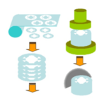
FEA defines the geometry as mesh that is a collection of elements divided into the finite element space for the analysis target (see Fig.2). The mesh model of the analysis target does not rely on selecting the geometry of the analysis target or the skill of the engineer because mesh can be generated using automatic mesh generation features if the geometrical data is available.
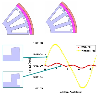 Fig.1 Comparing cogging torque for geometry with and without pits on the teeth ends
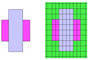 Fig.2 Geometry of an electromagnet model and mesh after discretization
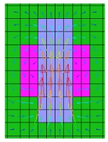 Fig.3 Magnetic flux density distribution of each element for the electromagnet model in Fig. 2.
2-b. Defining the Governing Equations
Maxwell's equations are the fundamental equations governing electromagnetic phenomena. These equations need to be treated accurately without approximation to achieve an analysis that can reproduce results obtained from actual measurements. Maxwell's equations are expressed by partial differential equations including time and space derivatives that are generally difficult to manually analyze correctly if the geometry is not simple with good symmetry. Analysis using numerical calculations is also required for an analysis that can account for the nonlinear magnetization properties and conductors.
FEA runs an analysis by applying Maxwell's equations to each element for the analysis model defining the geometry using mesh composed from many elements. As a results, an FEA analysis is run accounting for all of the phenomena, such as the eddy current distribution accounting for the flow of magnetic flux around conductors and the proximity effect in addition to the magnetic flux density distribution of magnetic materials and current distribution in conductors. The fundamental principle of FEA is directly applying the equations to a model of the analysis target to obtain the analysis results matching the measured values of a prototype.
An analysis accounting for the flux leakage is not impossible using the magnetic circuit method, but an analysis composing the magnetic circuit that accounts for the effects of the preliminary flux leakage is required. Therefore, the analysis accuracy varies according to the skill of the designer, but FEA can provide results without relying on the skill of the user because Maxwell's equations are applied uniformly to each element of the mesh generated for the analysis space.
2-c. Specifying the Material Properties
The magnetization properties change the output characteristics largely for devices including motors and transformers because they are constructed from magnetic material. The magnetization properties have nonlinear characteristics equivalent to the magnetic saturation. Analyzing the magnetization properties by accurately accounting for the nonlinear characteristics is vital to reproduce phenomena nearing the measured results.
An FEA analysis accounting for the actual magnetization properties using the nonlinear calculation method is expressed by the Newton-Raphson method (See Fig. 4). The magnetic flux density distribution when the complex magnetic flux density and excitation current varies with magnetic saturation can be obtained accurately because the results are obtained for the operating points of each element.
An analysis accounting for the magnetic saturation, even for the magnetic circuit method, is achieved by preparing a table of the magnetic resistance of each magnetic material for each excitation force, but it does not offer the same flexibility as FEA that supports arbitrary magnetic properties. An analysis accounting for the eddy currents is also possible by specifying the electric conductivity of the conductors to handle phenomena produced by eddy currents in conductors while including the effects of eddy currents in the magnetic circuit method is difficult because the distributions cannot be calculated.
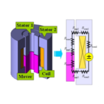
For example, the eddy currents produced in the core have a large effect on the response characteristics, such as relay switches. More will be introduced about this in the next issue. Qualitative evaluation becomes difficult for an analysis other than FEA when accounting for the eddy currents of the core in addition to the magnetization properties. The eddy current distribution and the response characteristics of the displacement for the core of the electromagnetic relay are indicated in Fig. 5 and Fig. 6.
These operating points are specific to the temperature dependency of the device because the effect of the raising temperature caused by the actual phenomena such as eddy currents. An analysis taking into account the temperature dependencies of the material properties, such as the electric conductivity, is necessary in these cases. Phenomena reproduced highly authentically when compared to the measured results can be expected because an FEA analysis accounting for the temperature dependency can be run by combining an FEA magnetic field analysis and an FEA thermal analysis. (There are also devices that proactively use the above phenomena including IH cookers)
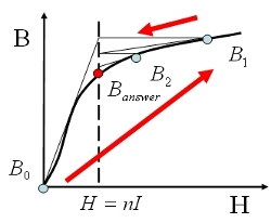 Fig.4 Convergence of the Newton-Raphson method
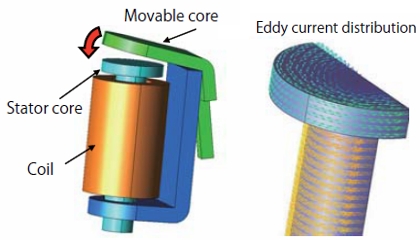 Fig.5 Eddy current distribution for a relay switch
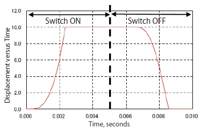 Fig.6 Response characteristics of the displacement for a relay switch
2-d. Specifying the Drive Conditions
The source of the magnetomotive force when handling electromagnetic phenomena is the magnets and current. Settings matching the actual operation environment and condition settings that have a high resolution are required to achieve a simulation that can authentically reproduce the physical phenomena.
The actual magnetization distribution can be reflected very near to the actual magnetization when using a magnet as the source of the magnetomotive force because the magnetization distribution can be defined by both the magnetization properties of the magnet and the complex magnetization pattern in each element using FEA. Simulations capable of high resolution settings such as FEA are vital to these evaluations because the magnetization of the magnets vastly affects the cogging torque waveform and the induced voltage waveform. Results comparing the cogging torque and the induced voltage when only the magnetization pattern of magnets in an SPM motor are changed is indicated in Fig.7. These results show a qualitative difference in the waveforms for varying magnetization patterns even though the magnetization is the same.
The current waveform is handled differently according to whether the waveform is known and unknown when the current is used as magnetomotive force. An analysis can be run by specifying the current values as values in a time interval table if the accurate time variations of the current are known. However, in most cases, a drive circuit including the power supply is attached to the analysis target and the current is determined by the analysis target as well as the drive circuit. An analysis using FEA that includes a circuit is required because the current waveform that needs to be specified is unknown in these cases. The circuit is closely defined using a circuit equation allowing an analysis to be run that comprehensively accounts for the drive by linking with FEA using Maxwell's equations to find a solution.
The time varying phenomena of the current before and after the charge and discharge of the capacitance when running an analysis of a solenoid valve including a drive circuit by linking to a circuit is indicated in Fig.8. The current following the LC vibrations caused by switching during the charge can be exported to a graph.
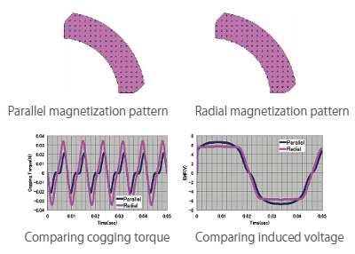 Fig. 7. Comparing the results for the cogging torque and induced voltage waveform
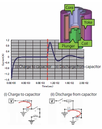 Fig. 8. Response waveform of current including a circuit (solenoid valve)
3. Conclusion
As described above, FEA is an analysis method that can accurately reproduced the measured results from the characteristics.
FEA does not simply obtain the electromagnetic phenomena based on Maxwell's equations, but also easily includes the affects of speed electromotive force produced by accounting for motion. A simulation reproducing the actual operation can also be realized by combining an analysis with an external circuit.
In the next issue, the effectiveness of FEA will be specifically examined through actual analysis examples which fully utilize the features that are available.
[JMAG Newsletter Summer, 2011]