Contents
1. Introduction
2. Excess loss modeling independent of frequency
　2.1 Modeling
　2.2 Identification of the excess loss coefficient \(C (B )\) and exponent \(\alpha\)
　2.3 Result of identification
3. Application of proposed model
　3.1 Other Conditions
　3.2 AC+7^th harmonic of different material
4. Summary
5. References

1. Introduction

Accurate loss prediction through simulation is crucial for high-efficiency advanced motor applications, especially in electric vehicles. The iron loss generated in the electromagnetic steel plate, one of the major loss components, consists of hysteresis loss, classical eddy current loss, and excess loss. Enhanced accuracy in simulation-based estimation of hysteresis loss has been achieved in recent years through the use of the Play model. Similarly, the use of the 1-D finite element method has enhanced the accuracy of the classical eddy-current loss prediction. However, the comprehensive modeling of excess loss remains challenging, and is an area requiring further investigations. Complex magnetic flux waveforms with multiple frequencies, such as minor loops, occur inside the motor, and modeling for such kind of waveforms is required.
Building upon the Bertotti model, this paper proposes a new modeling technique. More precisely, this approach is grounded in the power of the time derivative of the magnetic flux density and incorporates a flux density-dependent excess loss coefficient. First, we identify a combination of exponents and the excess loss coefficient that accurately reproduces the previously measured iron loss in a ring specimen. The obtained parameters are then considered to be material-specific and used in the simulation. For validation, the proposed modeling technique is applied as a case study to another material with AC + harmonic magnetic flux density.

2. Excess loss modeling independent of frequency

2.1 Modeling

The proposed model shares the general form of the Bertotti model by which the excess loss \(P_{ex}\) can be written as

(1)

where \(B\) denotes the magnetic flux density, \(t\) is the time, \(C\) represents the excess loss coefficient, and \(\alpha\) is an empirical exponent.
This section addresses excess loss modeling for arbitrary magnetic flux density waveforms, intended for use with electromagnetic finite element transient response analysis (FEA). We assume that \(C\) is a function only of \(B\) that is

(2)

In this expression, \(C (B )\)represents the flux density-dependent excess loss coefficient. The combination of the specific form of \(C (B )\) and the value \(α\) will be identified in the following section.

2.2 Identification of the excess loss coefficient \(C (B )\) and exponent \(\alpha\)

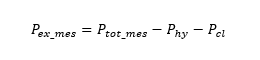
Using the measurement setup illustrated in Fig. 1, AC minor loop losses under DC bias are measured while changing the frequency of the AC excitation. The measurements were conducted with frequencies of 1 kHz, 5 kHz, and 10 kHz. The ring’s core material used was 35A210 electromagnetic steel sheets of which outer diameter 127 mm and inner diameter 102 mm, and its DC BH characteristic is given in Fig. 2. The measured excess loss \(P_{ ex }\)_{_}\(_ { mes }\) is defined as the difference between the total measured iron loss \(P_{ tot }\)_{_}\(_ { mes }\) and the sum of the hysteresis loss \(P_{ hy }\) and classical eddy current loss \(P_{ cl }\) from as expressed in Equation (3).

(3)

The hysteresis loss and classical eddy current loss are obtained through simulation using the Play model and 1-D FEA, respectively. These simulation approaches account for both skin effects and minor loop behavior. Two types of \(C (B )\) are compared: a constant value (hereafter called \(C_{ 0 }\) and a function with the shape based on the magnetic susceptibility of ferromagnetic materials, as shown in Fig. 2 (hereafter called \(C_\chi(B )\)). The exponents α are arbitrarily set to 1.5, 1.8, and 2.0, and for excitation frequency, the corresponding \(C (B )\), that best fits the measured iron loss is identified. Ultimately, a single combination of \(C (B )\) and \(\alpha\) should be selected for general application to arbitrary magnetic flux density waveforms, with minimal dependence on frequency.

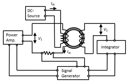
Fig. 1 Measurement system