Overview
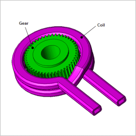
When hardening is performed, uniform heating is desirable, but there are significant factors to consider such as the geometry and arrangement of heating coils and the adjustment of current frequency and amount. When there are many design variables or items to evaluate, applying automatic computation using an optimization function for simulation can greatly reduce the workload.
In this example, an example of using an optimization function to design a coil to use for induction hardening a gear is presented.
Coil Design Variables
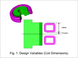
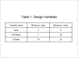
The coil has two turns, the distance from the center of the workpiece, CPosition, and the coil width CWidth are design variables. In addition, input current lamp is also defined as a design variable.
Fig. 1 shows the coil dimension design variables, and Table 1 shows all the design variables and range settings.
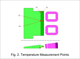
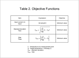
Fig. 2 shows the temperature evaluation points, and Table 2 shows the objective functions for coil optimization.The objective functions have the following three objectives.
- Minimizing input current
- Minimizing the standard deviation Tdev from the target temperature \(T_R\) using the evaluation point temperatures \(T_i\) (Fig. 2)
- Minimizing the bias Tbias from the target temperature \(T_R\) using the evaluation point temperatures \(T_i\) (Fig. 2)
Initial Design
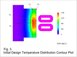
As shown in Fig. 3, the workpiece temperature is high at the temperature evaluation points T2 and T4 at the center of the workpiece, and low at the temperature evaluation points T1 and T3 near the end faces of the workpiece.
In the initial design, since the difference in temperature among the temperature evaluation points is large, improvements need to be made.
Pareto Curve Produced From a Multi-objective Optimization
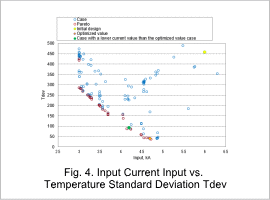
Optimization using a multi-objective genetic algorithm with a population size of 15 and 10 generations is performed. Fig. 4 shows a graph of input current Input and the standard deviation of temperature, Tdev, obtained by the multi-objective optimization.
The standard deviation of temperature, Tdev, one of the design variables with the objective of being minimized, is shown. The optimized value case, the case with the minimum Tdev value, may lower the input current value, and also reduces the standard deviation compared with the initial design.
Whether the current is lower after the optimization is checked. As shown in Fig. 4, if the current value is lowered, the temperature does not rise sufficiently at any of the four evalution points, and the standard deviation Tdev is larger.
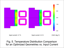
Fig. 5 shows a comparison of the temperature distribution for an optimized geometry vs. input current.
Sensitivity Evaluation Using a Correlation Matrix
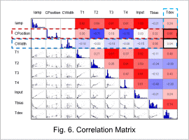
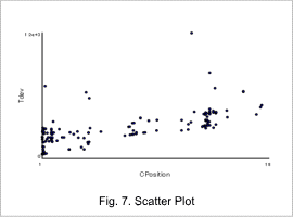
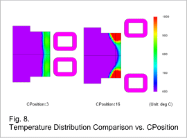
Fig. 6 shows a correlation matrix, Fig. 7 shows a CPosition-Tdev scatter plot, and Fig. 8 shows a comparison of two temperature distributions from two optimization cases with the same current where in one case Tdev is larger.
As seen in Fig. 6, CPosition is the most sensitive among the design variables, and the coil width CWidth has low sensitivity. In addition, as in Fig. 7, as CPosition increases, Tdev also increases.
From Fig. 8, it can be seen that as the coil positions move to the ends of the workpiece, the temperature also becomes higher near the ends of the workpiece and the temperature variation becomes larger.
From these results, it can be seen in this Fig. 8 example that CPosition has high correlation with Tdev, heating occurs more uniformly for cases when CPosition is small, and CWidth has low correlation with Tdev.
