Motor Design Course
This series features descriptions of our thoughts about motor design, targets beginning motor designers and provides information about design themes for those seeking to acquire basic knowledge about the subject. In the previous issue we discussed initial designs, arranging concept design plans as a starting point for detailed designs. In this edition, the third and last entry in the series, we will look at detailed designing for final designs.
Trade-offs are a key factor when it comes to detailed designs and they also happen to be areas in which JMAG-Designer and JMAG-Express excel. By describing case studies developed through trial and error while using JMAG-Designer or JMAG-Express we plan to provide hints that will help you move ahead with detailed design of motors.
Detailed Design of Motors
After completing a concept design and confirming that it satisfies requirements it's time to move onto detailed design of the motor. This is the real thing for motor designers. I've been using the term "detailed design," but I could put it another way and say it's a "final design." It's everything, right down to part costs and production. Without that much knowledge it's not possible to make an actual machine. Even if a design doesn't need to include a dimensional drawing, designers' thoughts should be directed to a point just short of that. Motor designers have to overcome the doubts borne by designers or motor technicians who will take the motor parts and use them to assemble the actual machines. Motor designers are the only people capable of overcoming those doubts. Designers will be asked things like "We've got to make this dimension 0.5 mm, but I can I make it 0.6 mm?" and respond, based on principle, by saying: "No, we'll make it 0.5 mm as it's supposed to be." "And here are the reasons why it has to be that way," before launching into an explanation for the reasons why the dimensions have to be the way they were designed. This is not something that applies only to motor design. We take this approach when it comes to developing software and a ramen noodle restaurant operator is doing the same thing when they propose adding a new item to their menu. The pain involved in the final stages of production is the most difficult to deal with.
My apologies for taking so long to go through the introduction and get to the point, but the key factors in detailed design are:
- Shaving away waste
- Scrutinize trade-offs and balance them with high-dimensionality
- Enhance quality
- Ensure a sufficient degree of reliability
Strictly speaking, none of these are standalone items, but as we move ahead while examining detailed design with these themes in mind, it all boils down to coming close to getting a decent product by keeping these matters in mind.
For this third part of the series I would like to move ahead with discussion of detailed design of motors while explaining typical examples of case studies using JMAG-Express Public or JMAG-Designer. Here are the conceptual design items written about in the first two editions (Table 1).
Table 1 Specifications Decided in the Concept Design
Shaving Away Waste
First, let's get rid of any waste. An example of an easy to understand waste is a magnetic path with extremely low levels of magnetic flux density. Getting rid of these areas lightens the work. Alternatively, sorting coil circuits may reduce copper loss. However, in reality in most cases there is rarely ever a great deal of unconditional waste and that means there are often trade-off problems results from cutting into breathing space.
Magnetic paths inside the rotor can be given as an example of waste that's easily overlooked. The shaft needs to be checked and verified, so there's value in giving it an examination because you don't want to shave off more than necessary due to the magnetic path. Above all make sure you have the minimal space needed for the magnetic path (Fig. 1).
In our concept design the shaft diameter was 16 mm and we allowed another ±8 mm scope to this. Enlarging the shaft diameter means narrowing the rotor magnetic path.
 Fig. 1 Examining the Shaft Diameter
Look at the difference in shaft diameter affects the correlation between the rotor weight and torque constant and between the speed-torque characteristics (Figs. 2 and 3). As a result of allowing for the shaft diameter (hole diameter), even though we are narrower than the 16 mm of the concept design, it didn't enhance the torque constant. This is because we were showed that the magnetic resistance within the magnet had an initial value that was low enough that boosting the magnetic paths would only increase weight and create waste. Alternatively, raising the number to 20 mm had almost no effect and widening up to 24 mm did not leave enough room for the magnetic path within the magnet, which dropped the torque constant.
We now know that if the shaft hole diameter can be widened from 16 mm to 20 mm without adverse effect. Incidentally, the rotor core weighs 235 g, but we can lighten this by 40g to make it 191 g. In a motor with an overall weight of about 2kg, this may seem an insignificant contribution, but waste is waste, so we'll change it to 20 mm.
 Fig. 2 How Shaft Diameter Differences
affect the Rotor Weight-Torque Constant Relationship
 Fig. 3 How Shaft Diameter Differences
affect Speed-Torque Characteristics
Scrutinizing Trade-offs
The most challenging aspect of design comes in the trade-offs. Something working out may mean something else no longer working out, so fixing up clearly contradictory design parameters is the designer's job.
Here, we'll examine the yoke width in the stator core. If you fix the outer diameter and stack length, there'll be almost no impact on the overall outer layer or weight. One of the items a motor designer must examine is being adept at achieving balance in the motor interior. Thickening the core-back reduces the risk of magnetic saturation, but it also applies pressure on the coil winding space and increases the resistance and copper loss. Making the core-back has the opposite effects. To appropriately control copper loss, study dimensions to get them right and avoid magnetic saturation, which is a prime example of a trade-off, arrangement and compromise.
We changed the initial core rear value of 8 mm by ±2 and examined it (Fig. 4). At the same time we changed the wire diameter to maintain the coil at 60 turns and lamination factor at 50.4%, synchronizing this with only the resistance. Show Parameters (Table 2).
 Fig. 4 Examining the Core-Back
Table 2 Wire Diameter and Resistance in the Core-Back Width
Let's check up on what happens to the relationship between resistance and the torque constant when you change the core-back width. Increasing the concept design's 8 mm does not change the torque constant, so we know that we still have room to move in regard to the magnetic path if we use the initial values (Fig. 5). And we also learn that resistance decreases the slot area, which increases linearity and shows that widening the core-back from its 8 mm has not benefit. But if we narrow this, the torque constant drops the more we reduce the width and it starts to show an effect on the magnetic path. You can confirm also that when it comes to resistance, linearity decreases.
 Fig. 5 How Core-Back Width
affects the Resistance-Torque Constant Relationship
Checking out the speed-torque curve depending on differences in the core-back width shows few characteristics at 7 mm to 10 mm, but at 6 mm, you can confirm signs of the maximum torque dropping (Fig. 6).
 Fig. 6 Speed-Torque Characteristics Depending on
Differences in the Core-Back Width
Now looking at the speed-efficiency characteristics reveals that efficiency increases in conjunction with the decreased resistance that results from narrowing the core-back, but lowering it beneath 7 mm shows almost no difference (Fig. 7). Integrating all these factors leads to changing the core-back width to 7 mm.
 Fig. 7 Speed-Torque Characteristics Depending
on Differences in the Core-Back Width
Next, let's examine teeth width. Positioning on the magnetic path is the same as the core-back width, which enables expanding the coil area through narrowing the teeth width, which raises expectations of being able to decrease resistance, but also heightens the risk of magnetic saturation. And that means the focus of our examination should be achieving a balance between resistance and magnetic saturation. In the concept design, the teeth width was 5 mm, so we will add another ±2 mm to its scope (Fig. 8).
 Fig. 8 Examining Teeth Width
Taking a look at the resistance-torque constant relationship while changing teeth width makes it easy to understand that changing the teeth width had a trade-off relationship with resistance and magnetic resistance (Fig. 9). Narrowing the teeth width from 4 mm to 3 mm drastically boosts magnetic saturation and the torque constant is lowered. On the other hand, there is no change in the torque constant from 6 mm to 7 mm, which looks space to maneuver on the magnetic path. Checking the teeth shows that even with average magnetic flux density it still achieves 1.8 T at 4 mm and that the ordinary saturated magnetic flux density of silicon steel sheets is approaching 2.0 T (Table 3).
 Fig. 9 Resistance and Torque Constant due to Teeth Width Differences
Table 3 Teeth Width and Average Magnetic Flux Density (Teeth)
Looking at the speed-torque characteristics after changing the teeth width we learn that the torque constant hasn't changed after 5 mm or more, so there is almost no variation in the maximum torque (Fig. 10). But we also learn that narrowing by 4 mm or 3 mm will reduce the maximum torque.
 Fig. 10 How Differences in Core-Back Width affect Speed-Torque Characteristics
As reducing the torque constant is the equivalent of lowering the induced voltage constant, gaining a grasp of the output properties at high rotation would seem to have some appeal from a design viewpoint, but if you're looking for high rotation, a better and more correct approach to achieve this would be to reduce the number of coil turns and magnet weight. With the benefit of some magnetic flux, there's no benefit in spoiling it by making the teeth more detailed.
Now, let's check on the thickness of the magnet. It goes without saying that you need to carefully scrutinize how much you use NaFeB magnets in particular, as their material cost is extremely high compared to other motor parts.
Thickening the magnets increases magnetomotive force within the magnet itself. However, as the magnet's relative permeability is almost 1.0, when it comes to the motor's magnetic path, thickening the magnet also expands the air gap by the same amount of thickness added, which ups the magnetic resistance across the entire magnetic path and there is not an increase in the amount of magnetic flux equivalent to the increases thickness. The conceptual design was 4 mm, but let's look at it with a scope of an additional ±2 mm (Fig. 11).
 Fig. 11 Examining Magnetic Thickness
Take a look at the relationship between magnet thickness and magnet weight (Fig. 12). Making the magnet thicker than the concept design doesn't increase the torque constant. As stated earlier, this boosts magnetomotive force and magnetic resistance. On the other hand, making the magnet thinner greatly reduced the torque constant. A motor's magnetic path contains a rotor, stator and air gap, as well as the magnet. Making the magnet thinner makes the unchanging air gap relative thickness relatively more effective, so you can conform how making a magnet thinner greatly affects the torque constant. A check of the speed-torque characteristics shows that a change in the torque constant will leave output characteristics expressed in the same manner (Fig. 13).
 Fig. 12 Magnet Weight and Torque Constant Depending on Magnet Thickness
 Fig. 13 Effect of Different Magnet Thicknesses on Speed-Torque Characteristics
After a check of the relationship between magnet thickness and speed-torque characteristics, we can confirm that it's probably best to thin the concept design's 4 mm down to 3 mm. But to decide on the actual thickness to use, you must allow for factors like irreversible demagnetization and thermal demagnetization. Calculation accuracy is crucial for this kind of analysis, so using a highly precise software like JMAG-Designer would be a wise choice.
With conventional motor design there are also sorts of other trade-offs that need to be considered, but writing all of them would require an entire book in itself, so I'll leave talk about trade-offs here and move onto our next theme, which is enhancing quality.
Enhancing Quality
For the purposes of this exercise, we'll regard quality as being the reduction of torque variations, like cogging torque, and the causes of vibration. Cutting both of these will lead toward improved quality.
For example, run a sensitive solver like JMAG-Designer for geometries like cogging torque. Here, we can confirm how cogging torque will change according to the angle parameters used for the magnetic pole's arc. JMAG-Designer analysis windows are packed with settings parameters or results analysis even though it is intended for general purpose use and these capabilities enable running highly accurate analyses (Fig. 14).
 Fig. 14 Examining Magnet Angle
Analyze the obtained cogging torque waveform (Fig. 15). In the concept design the angle at the magnetic pole was 80 deg with intervals at 10 deg. The cogging torque at this time was ±0.65 N·m. Narrowing the magnet angle broadens the intervals and drops the cogging torque, enabling confirmation that narrowing to 68 deg will lower it to ±0.15 N·m. But narrowing it any more than this will, conversely, increase the torque variations.
 Fig. 15 Cogging Torque Waveform
Narrowing the magnet angle to cut the cogging torque will naturally also reduce magnetic flux, which connects to a lower torque constant. Obtained the induced voltage waveform (Fig. 16) at this time from JMAG-Designer. The number of rotations is 600 rpm.
A feature will be that amplitude in the induced voltage waveform will be in the vicinity of 14 V and there will be no great difference. With this waveform you can see that it's biggest near the square wave where the magnetic arc angle is largest and the higher components increase as the angle gets smaller. When the cogging torque reaches its smallest figure of 68 deg, the maximum has increased to 15.5 V, while at 60 deg it lowers to 12 V. Drastic changes in induced voltage such as those seen here makes it hard to maintain sinusoidal waves in the current and becomes a cause of iron loss, so it's a factor requiring plenty of caution.
 Fig. 16 Induced Voltage Waveforms Above: One period, Below: Peak Vicinity
Now let's analyze the results of FFT processing of the induced voltage waveform (Fig. 17). Changing the magnet angle from 84 deg to 64 deg lowers gap flux linkage to 78% in a simple conversion. Coinciding with the narrowing of the voltage amplitude in the waveform of 20 Hz is gradual reduction that will lower voltage from 17.5 to 15.8 V, but 91% will be retained. However, the 60 Hz component, which corresponds to the slot harmonics, will drop from 4.6 V to 0.6 V, a significant decrease of 14%. However, after a temporary downturn through five rotations of the 100 Hz component, it showed signs of moving upward rapidly and ultimately doubled from 1.8 V to 3.3 V. In this manner, the motor has qualities unable to be read in the waveform alone, which means that ultimately the only item capable of providing a decision is a highly accurate tool.
 Fig. 17 Induced Voltage Vector Comparison for Each Magnet Angle
Is this Reliable Enough?
You've ensured the performance, raised the quality and now all that's left is reliability. We're talking about electric machinery, so it's only natural that it has output, but to be useful in the real world, it has to have a stable and reliable performance in a variety of environments, such as remaining trouble-free despite vibration and shock. These matters should be pretty much solved during the initial examination and concept design stages. Naturally, if it breaks there's a problem, but in addition to that, having too much room to move is also an issue from a design viewpoint.
Here, let's check how properties changed within the temperature range. I'm writing this in February 2014. I recently heard a news story about how the temperature had fallen below -30 deg C in Japan's northernmost island of Hokkaido. But in summer, you will hear news stories of how the temperature topped 40 deg C in Shikoku. Even in a small country like Japan, temperature variation spans -30 deg C through to 40 deg C, so a motor must be able to perform properly within that range. Let's check how performance varies at 20 deg C ±40 deg C.
The magnet and coil are among the parts most powerfully influenced by the motor. The temperature coefficient of a residual magnetic flux density Br of a neodymium magnet is said to be -0.11%/K and we know at variation of ±40 deg C, the Br will change by ±4.4%. Similarly, the coil's electric conductivity temperature coefficient is said to be 0.38%/K and at ±40 deg C variation, we discover that it changes ±15.2%.
The image shows how, when applied to a motor, differences in temperature change the torque constant and coil resistance value (Fig. 18). Say the initial temperature is 20 deg C, raising the temperature to 60 deg C will increase coil resistance and loss, prompting the synergetic effect of reducing output and efficiency as the magnet weakens and causes the torque constant to drop. There is an impact on the torque constant, which is decided by magnetic strength, but we learn that there is significant change in the copper loss with a large temperature coefficient. Conversely, dropping the temperature to -20 deg C raises the Br and lowers the resistance, leading to expectations of the properties enhancing.
 Fig. 18 Temperature Variations in the Torque Constant and Coil Resistance
Next, let's check what kind of an effect occurs on motor properties. Looking at speed-torque characteristics, the torque constant has decreased, enabling a check at peak current (Fig. 19). On the other hand, when the magnet's magnetic field weakens the induced voltage constant also goes down and revolves at high speed. With speed-efficiency characteristics there is a decrease in efficiency due to increased copper loss brought about by rising temperature (Fig. 20) This is especially so during output when copper loss is controlling, which keeps speed low and decreases efficiency, and we can see that 20 deg C at 75 % efficiency will fall at 60 deg C to 70 % efficiency.
The effect of this is being able to generate your own heat during actual operations. If trying to maintain motor output at a certain point, you can get caught up in the following sequence of events, which will dramatically raise the temperature. As temperatures increase, the motor temperature rises → decreased performance and efficiency → recovery through increased input → increased heat generation → motor temperature increases even further. It's really important to check whether performance exceeds objective indices at times of high temperature.
 Fig. 19 Speed-Torque Characteristics and Temperature Differences
 Fig. 20 Speed-Efficiency Characteristics and Temperature Differences
Did You Achieve What You Aimed For?
These detailed designs polish proposed designs. Did you easily satisfy requirements and get an idea about reliability and costs? If so, your design is now complete.
Though only examining a few designs, we reviewed each part of the concept design. Here are the changes (Table 4). We made slight improvements to operations as a result of our examinations. Most noticeable of these improvements was being about to reduce the size of the magnet, which was effective from the cost-cutting perspective.
Table 4 Concept Design and Final Design
Looking at the N-T curve and speed-efficiency characteristics, we lowered the peak torque in the final design from 3.03 N to 2.90 N·m and the efficiency has improved marginally. In addition, as there has been a decrease of at least 20% of the magnet, it's probably not a bad result (Figs. 21 and 22).
Of course, we've only examined one area for the purposes of this magazine, so with the actual design far greater scrutiny must be given to a lot of other areas. I don't think a single examination will lead to improvements of several percentage points, either. At best, it would probably be about 1%. But, just as an old saying goes that "little and often fills the purse," a 1% improvement in many items can be expected to improve the product several percent overall, so it's important to keep plugging away.
 Fig. 21 N-T Curve in the Concept and Final Designs
 Fig. 22 Speed-Efficiency Characteristics in the Concept and Final Designs
Utilizing Feedback from the Prototype
When the final design is completed and designs all put in place it's time to move onto the prototype to verify answers. There are many things involved here, so they need to have a further countermeasure. TO make it easily understandable, you may get a calculation result where the design (analysis) says torque of XX N·m was output, but in actual machinery, there are times when it may have stopped at YY N·m. Looking into the cause of that difference can only be done as a countermeasure, but the process of formulating this is also an opportunity to examine what point a problem occurs or where an error arises, so this is extremely vital feedback. Once you have gained a grasp of what has gone wrong, it's possible to apply corrective measures to the examination method and improvements will become clear. Veteran designers have built up a multitude of this kind of experience. Putting aside in advance a few percent for performance margin and then spitting out a number toward the end while gambling on the material factor is perhaps one way that they tackle things with their accumulated know-how.
Series End
This article is the final issue in this series on our thoughts about the process of designing motors. I think the series probably gave those starting out in motor design or people simply interested in the issue some sort of an idea of what happens. Have these articles helped you with learning about how to use the tools in JMAG-Express Public or JMAG-Designer as part of the design flow?
However, when it comes to design, the contribution made by tools is pretty much on a par with an easy to use calculator. To make a good design undoubtedly requires a designer with a great sense of designing. Even if a designer chooses to get help from a tool, the tool alone will not be able to create a great design plan. Perhaps optimized design plans created with a combination of optimization software and magnetic field analysis software will still not be as good as a design plan cranked out by an experienced designer. But expectations of an even better plan are possible when a veteran designer uses optimization software, so beginners will always lose out to long-term designers regardless of the tools they may use. Consequently, the only approach for beginners to take is to throw yourself into learning and polishing your skills with constant production and eventually become a veteran designer in your own right. Please use JMAG-Express Public or JMAG-Designer as the venue to polish your skills and designing awareness.
(Yoshiyuki Sakashita)
Column: What Happens when Torque Variations Arise?
The Motor Design Course focused on motor design, but this column picks up issues that could not be fully covered and looks at them while conducting a simple experiment.
In this issue, we will look at torque ripple. Cutting torque variation is an issue motor designers deal with in perpetuity. Unfortunately, we don't have enough design strength to be able to give you information that will work like magic or be like some secret plan to solve your problems. What we can do, though, is show you how to use JMAG to display torque variations in the hope it may provide you with a hint about how to devise measures to reduce torque variations.
First, how does a motor generate torque? Have you ever seen torque (or electromagnetic force)? I haven't. Textbooks will say things like "Lorentz force generates torque" or "Maxwell stress makes it build up," but all this is only ever in a book. I'm always thinking about how I've never actually seen torque. I can't get rid of this feeling even now, but JMAG gives us the opportunity to see something close to torque being generated.
 Fig. 1 Motor Model Geometry
We ran an analysis on an IPM motor to observe how torque variation is generated (Fig. 1). The analysis was on a model with 4 poles and 24 slots and an electric angle of 90 deg. Passing a 3-phase sinusoidal current through a current results in a torque waveform like the one shown in the image (Fig. 2). Looking at the torque waveform graph shows significant dips in torque variation every 15 degrees and you can predict there will be a slot pitch effect. If you quickly come to the conclusion at this point that it's going to be possible to predict slot pitch effect, you're not going to see the torque ripple. We need to dig a little deeper.
 Fig. 2 Motor Torque Variations
Check the motor flux lines and nodal force in a state where torque is being generated normally (Figs. 3 and 4). What stands out is just how extremely large size of the rotor and stator attraction force (the radial direction force). But, the radial direction force doesn't contribute to torque, so we can ignore this.
Looking at the electromagnetic force vector from the teeth tip shows that in the teeth near the boundary between the motor's N and S poles and joined to the torque there is significant force in the Į direction. There is apparently no effective torque being generated from teeth in other positions.
 Fig. 3 Magnetic Flux Lines and Nodal Force Vector Plots in a Motor
 Fig. 4 Magnetic Flux Lines and Nodal Force Vector Plots in a Motor (Enlarged)
Next, set the torque conditions for each tooth and observe the torque for each tooth (Fig. 5).
 Fig. 5 Overall Torque Waveforms for Each Teeth (Electric angle half period)
You can make a really rough estimation from the image stemming from the nodal force vectors, but plotting these on an actual graph is extremely tough. Solving using this information shows a significant portion of the torque generated in the motor comes from a single tooth. It's easy to see that switching the tooth in conjunction with rotations will continue generating torque. Focusing on a single tooth gives the impression that torque is generating over a roughly 15-degree stretch of the 90-degrees making up a half period of the electric cycle, leaving the remaining 75 degrees essentially idle. The "roughly 15 degrees" here is important because torque variations in this "roughly" area are large and we learn that troughs are created when overlapping doesn't work well.
Let's take a slightly more detailed look at torque waveforms. This is an enlargement of the 0-15-degree area equal to a single teeth pitch phase (Fig. 6).
 Fig. 6 Overall Torque Waveforms for Each Teeth (1 slot)
It goes without saying that we are led to the conclusion that the key to reducing torque variations lies in skillful overlapping. It would be ideal if it was possible to increase the peaking time, but I think the reality would be more likely to involve imagining measures that fill in a trough created by breaking down a peak. A measure like this would have an effect on actual model geometries like slots, rotors or detailed geometries thus it would be impossible to examine without using a high-precision finite element analysis (FEA) like JMAG-Designer.
We used an IPM motor in this case. I think results would turn out differently with an SPM or concentrated winding (fractional slots). I'm really interested to see what would happen with an induction motor. This is a real test for designers, but we expect that designers will be able to put JMAG to use to come up with solutions.
[JMAG Newsletter March, 2014]