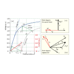
Fig. 1 Some common operating characteristics of synchronous machines
The wound-field synchronous machine was one of the first electric machines to benefit from the development of numerical field-analysis techniques in the 1960s [3]. Since then, the technology of electromagnetic field analysis has developed from its beginnings in the limited solution of nonlinear boundary-value problems to systems of ‘all-powerful’ simulation software covering many branches of physics and engineering. In the early days, field solutions were helpful in the process of design and in performance calculations, but their role was auxiliary or supportive, in contrast with the central role of simulation software today. Number-crunching facilities were a fraction of what we have today, while graphics display technology was rudimentary.
Because of its widespread use and great economic importance, it was common to calculate or measure standard operating characteristics for the synchronous machine (and in fact for all types of machine). Graphical methods were the norm, as they are today: but with a difference. In the early days, graphs were calculated and plotted by hand. Because of the high cost in both skill and labour, these operating characteristics were precious. They could not be easily reproduced if lost, or in the event of design changes or system changes. So we can regard them as ‘canonical’ records of the machines and systems of the time.
The evolution of analysis methods raises some questions about the operating characteristics. If we have all-powerful simulation software, why do we need them? Why can’t we just calculate whatever we need, whenever we need? What’s wrong with a strategy of ‘simulate on demand’ or ‘instant simulation’ for all the performance calculations that might be required?
I won’t attempt to answer that. What I will try to do is to list and describe some of the most important operating characteristics. There are several sources relevant to this topic. Classic texbooks all cover them in detail [4–9], while there is a vast archive of journals and conference proceedings (see [10], for example). They are mentioned in standards [13] and grid codes, and are likely to be found in specification documents and contract documents.
Fig. 1 shows a collection of some of the most common operating characteristics. A second question arises, as to the best methods for calculating them, and whether the finite-element method can be used.
It might be thought that the list should begin with the open-circuit characteristic (OCC), the short-circuit characteristic (SCC) and perhaps the zero-power-factor characteristic (ZPFC). However, these are put aside as belonging to the set of basic tests intended to determine machine parameters, rather than operating charactertistics per se.
All of the material in this Engineer’s Diary is covered in greater detail in Videos 69–73.
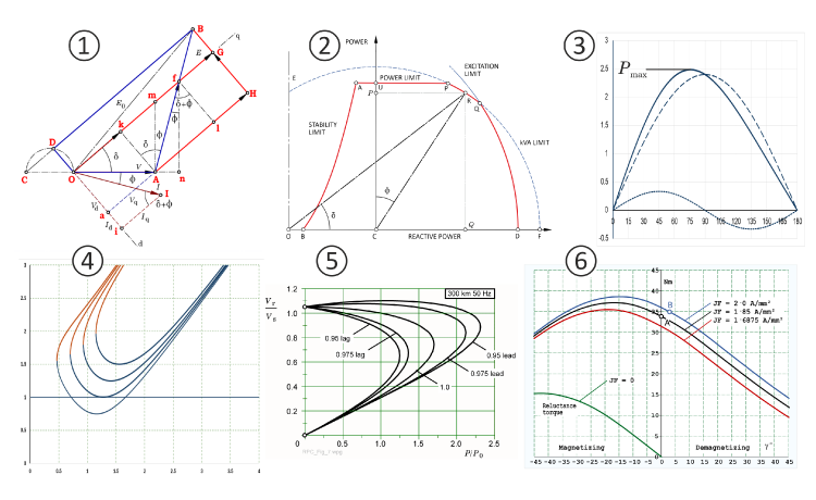
1. The phasor diagram provides the theoretical basis for almost all the steady-state operating characteristics, with good reason. It encapsulates the essential operating theory of the synchronous machine in the steady state, in which patterns of sine-distributed flux and ampere-conductors resolve themselves into sinusoidal time-waveforms of voltage and current at the terminals. This is the basis of the Potier diagram and of Blondel’s original two-reaction theory of the salient-pole synchronous machine, both of which date back to the 1890s. The relationship between spatially-distributed field quantities and the time waveforms of flux-linkage, voltage and current depends on the principle of sinusoidal distribution, and this applies not only in the actual reference frame but also in dq axes, αβ axes, and in space-vectors. To the extent that harmonics exist in the spatial distributions of flux and ampere-conductors or in the time-waveforms of flux-linkage, voltage and current, the theory relies on the fundamental harmonic obtained by Fourier series analysis (not the FFT). In such cases the harmonics are usually dealt with by means of differential leakage reactance, or treated separately as parasitic effects outside the sphere of the core theory.
The phasor diagram will be covered in Engineer’s Diary No. 92, but we can make two additional points. First, it provides simple equations consistent with the equivalent circuit, usually expressed as complex numbers or as components in dq axes. Secondly, the classic works drew out of the phasor diagram a number of modifications permitting the calculation of transients and certain fault conditions, mainly by substituting transient or subtransient reactances in place of synchronous reactances.
The use of the term ‘reactance’ is inherently rigorous with the phasor diagram and with all things derived from it, because the phasor diagram is based on fixed-frequency operation; and since it deals with voltages and currents, it is logical to treat inductive (and capacitive) elements in terms of their reactances in [ohm], and not in terms of inductance (or capacitance) which are better adapted to time-dependent transient equations and phenomena. Of course the relationship between reactance and inductance is very simple: X = 2πƒL for an inductive element. But the simplicity of this relationship tends to hide certain complications, because in the steady-state calculations that use reactance, X is expected to be constant, or at least to vary in a relatively gentle manner with current; whereas L is liable to vary much more wildly, and even its definition may be a matter of dispute (incremental vs. total inductance, etc.).
2. The kVA chart (sometimes called the MVA chart or the reactive capability chart, or just the operating chart), is a diagram showing the power P and reactive power Q at a glance, at any operating point. It is obtained by a geometric construction based on the phasor diagram, which produces a polygon of currents rather than voltages; these are scaled by the terminal voltage to give a chart plotted in units of kW on the vertical axis for P, and kVAr on the horizontal axis for Q. (See [10]). Sometimes the axes are interchanged. There are even real-time instruments on the control panels in power stations showing the instant-by-instant operation of the station and its generators in terms of this chart.
The kVA chart generally includes operating boundaries or limits set by the maximum permitted kVA (this is really a current limit and therefore a thermal limit); the maximum excitation (field current); power (the limit of the prime mover); and stability. This is obviously useful in a generating station supplying a load that may vary from heavy inductive loading during the daytime, to low-power capacitive loading (of transmission lines) at night.
3. The power/angle characteristic is a graph of power versus load angle δ, where δ is the phase angle between the terminal voltage and the open-circuit voltage. It is axiomatic that the power transfer between two AC voltage sources E and V goes with (EV/X) sin δ, where X is the series inductive reactance. This formula applies directly to round-rotor (nonsalient-pole) machines; for salient-pole machines there is also a second-harmonic term in δ which is associated with reluctance torque, and which depends on the difference between Xd and Xq. For synchronous motors the torque would normally be plotted instead of the power, but the curve retains the same shape (small differences due to losses being ignored in this assertion).
An important feature of the power/angle curve is that there is a maximum transmissible power that depends on the synchronous reactance and the repsective voltages E and V, and not on the prime-mover or any other properties of the system. This maximum power is called the steady-state stability limit. If for some reason a generator were driven with a mechanical prime-mover to a power level approaching the steady-state stability limit, it would become unstable, in the sense that small changes of δ would be slow to attenuate, and larger changes (caused by inevitable transients in the system) might tip the operating point over the peak of the curve; this could result in the loss of synchronism and pole-slipping, which must be considered as dangerous malfunctions. The excitation (and therefore the generated voltage E) can be modulated dynamically by the AVR (automatic voltage regulator, i.e., the controlling element in the field-current supply) to help stabilize the operation and prevent small oscillations of the load-angle δ. Above a certain level, these oscillations are physically observable and they are called ‘hunting’. It is one of the functions of the damper bars (amortisseurs) to attenuate such oscillations by means of dissipation though induced currents in their closed circuits on the rotor; but the effectiveness of the amortisseur is passive and not at the same level as the control provided by the AVR.
The power/angle characteristic is used in the analysis of faults in the transmission and distribution system, in which a change of effective reactance between the generator and its load is represented by a different power/angle charecteristic (usually at a lower maximum power, higher effective reactance). Then the equal-area criterion [7] can be used to analyse the response of the generator to a fault, and to determine the necessary fault-clearing time for safe recovery.
4. V-curves are curves of armature (stator) current versus field current, usually at constant terminal voltage, with contours of constant power and/or power-factor superimposed. They show the excitation required to minimize the armature current (corresponding to operation at unity power-factor). They also show the operation in stable and unstable regions depending on the value of the load-angle δ. Obviously only the stable regions can be used. The V-curves are so named because of their shape.
5. Voltage regulation curves show the variation of terminal voltage at the ‘receiving end’ or ‘load end’ of a circuit (such as a transmission line) connecting the generator to a load that is characterized by its power and reactive power, P + jQ. These curves clearly show the effect of inductive loads in reducing the load voltage, and of capacitive loads in raising it, giving rise to several related theorems and principles in the reactive compensation of transmission lines, [14]. They also show the Ferranti effect that is observed on long lines, in which the receiving-end voltage at no-load increases above the sending-end voltage, due to the charging current flowing in the distributed shunt capacitance of the line.
6. Torque / excitation curves can be plotted for a synchronous motor, as a means of determining the optimum combination of field current and armature current (including the control phase angle in inverter-fed synchronous motor drives). A detailed example is given in [1].
Further reading
[1] Hendershot J.R. and Miller T.J.E., Design Studies in Electric Machines, Motor Design Books LLC, 2022, (Blue Book)ISBN 978-0-9840687-4-6, sales@motordesignbooks.com [2] Hendershot J.R. and Miller T.J.E., Design of Brushless Permanent-Magnet Machines, Motor Design Books LLC, 2010, (Green Book)
ISBN 978-0-9840687-0-8, sales@motordesignbooks.com [3] E. A. Erdelyi, S. V. Ahamed and R. E. Hopkins, "Nonlinear Theory of Synchronous Machines On-Load," in IEEE Transactions on Power Apparatus and Systems, vol. PAS-85, no. 7, pp. 792–801, July 1966, doi: 10.1109/TPAS.1966.291707. [4] Say M.G., The Performance and Design of Alternating Current Machines, Pitman, London, Second Edition, 1948 [5] Kostenko M. & Piotrovsky L., Electric Machines, MIR Publishers, 1974 [6] Bewley L.V., Alternating Current Machinery, Macmillan, N.Y., 1949 [7] Kimbark, E.W., Power System Stability, Wiley, New York, 1948 [8] Clarke, Edith., Circuit Analysis of A-C Power Systems, John Wiley & Sons, 1943 [9] Jones C.V., The Unified Theory of Electrical Machines, Butterworths, 1967 [10] Walker J.H., Operating Characteristics of Salient-Pole Machines, Proc. I.E.E. - Part II: Power Engineering, 100 (73), 1953, pp. 13–24. doi:10.1049/pi-2.1953.0004 and J.I.E.E., Vol. 112, No. 2, 1953. pp. 13–23 [11] Doherty R.E. and Nickle C.A., Synchronous Machines I — An Extension of Blondel’s Two-Reaction Theory, Transactions A.I.E.E., June 1926, 912–947 [12] Potier A., Sur la réaction d’induit des alternateurs (On the armature reaction of alternators), l’Éclairage Électrique (Paris), Vol. 24, 1900, pp. 133–141 [13] IEEE Standard 115:2019, 67:2005 [14] Miller T.J.E. (Ed.), Reactive power control in electric systems, John Wiley & Sons, 1982. ISBN 0-471-86933-3