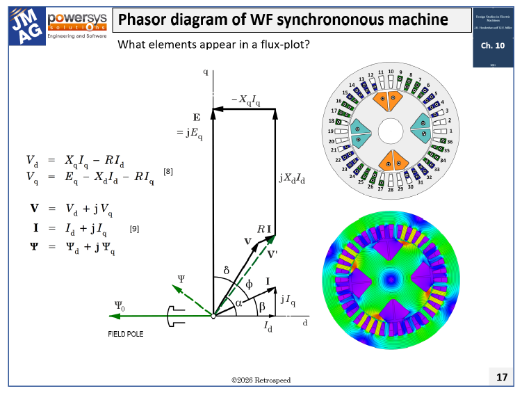
Fig. 1 Phasor diagram of wound-field synchronous machine: generating, overexcited
The phasor diagram is fundamental in the theory and calculation of the steady-state operation of the synchronous machine (including both wound-field and permanent-magnet types). This is not simply a matter of convenience or convention: it is due to the fact that it represents the correspondence between spatially sine-distributed quantities around the air-gap (flux and ampere-conductors) and time-dependent terminal quantities (flux-linkage, voltage, and current) with nominally sinusoidal waveforms. This correspondence pertains strictly to the fundamental space-harmonic and time-harmonic components of the relevant quantities, implying steady-state operation which is naturally expressed in terms of complex numbers, i.e., phasors.
We have seen in Engineer’s Diary No. 91 that most of the standard operating characteristics and charts for synchronous machines are calculated in the classical theory from the phasor diagram. Also, the Potier diagram (Engineer’s Diary No. 90) explicitly combines the the time-related phasor diagram with the space-related MMF diagram, complex numbers being used in both parts for calculations.
It is also relevant to mention space-vectors, which rely on the assumption of spatial sine-distribution of flux and ampere-condutors, but which make no restriction on the time-waveforms of terminal quantities (flux-linkage, voltage, and current); therefore the space-vector is not a priori a steady-state quantity, although it retains its definition under conditions of steady-state AC operation.
With this background, the question arises, What elements of the phasor diagram appear in a flux-plot? — or, more generally, What is the relationship between a finite-element flux-plot and the phasor diagram, or a space-vector diagram?
Imagine the following thought-experiment, in which we start with a machine cross-section and a finite-element flux-plot for a particular load; both these graphic images are included in Fig. 1. It is not possible to draw the phasor diagram for that load condition directly from the flux-plot: further processing steps are necessary.1 These are considered as follows.
- The phasor diagram depicts terminal quantities (voltages, currents, and sometimes flux-linkages), whereas the flux-plot depicts distributed quantities (flux density, current density). Fortunately JMAG has inherent facilities to produce terminal quantities: terminal current is related to the distributed current-density via the winding editor and related pre-processing functions; terminal flux-linkage is obtained from the line-integral of vector potential around the entire length of any closed winding.2
- Resistive voltage-drops are obtained by multiplying the current by the winding resistance. But induced voltages require the time-derivative of flux-linkage (Faraday’s law),3 and unfortunately a single static flux-plot is frozen at one instant in time. If the time-waveform of all currents is known, and if the rotor position is also known as a function of time, then it is possible to compute the waveform of terminal flux-linkage by means of a series of static finite-element computations, performing the necessary differentation afterwards. If, on the other hand, the terminal voltages are known, but not the currents, a more complex finite-element process must be used, in which the currents will be part of the solution and not the input. If, in addition, the rotor position is not known a priori as a function of time, the finite-element process must be linked to a mechanical simulation of the rotor and whatever is coupled to it. We can develop this line of thought to include cases where transient temperature changes (and consequent changes in material properties) are important; in such cases the process must also include a thermal simulation. The need for ‘multi-physics’ capability quickly becomes apparent.
- Assuming that the time-waveforms of all flux-linkages (and hence all terminal voltages) have been made available by one or other of these processes, we are still not ready to draw a phasor diagram. That’s because the voltages and currents are at this point in the form of time-waveforms: i.e., arrays of instantaneous values that could be plotted on a graph. A phasor, however, shows the root-mean-square value and the phase angle of the fundamental time-harmonic component, which must be obtained from the corresponding time-waveform by Fourier series analysis (not the F.F.T.) Phasors are defined for pure sinewaves and, strictly speaking, they are valid only for steady-state conditions with no harmonics.
- A final stumbling-block is that the phasor diagram shows quantities that do not co-exist simultaneously. For example, the terminal voltage V would be measured on-load, but the open-circuit voltage E must be measured on open-circuit — a completely different condition that does not and cannot co-exist simultaneously with the on-load condition. This has profound implications for the usage and validity of the phasor diagram, and for all calculations and characteristics derived from it, including (for example) torque calculations. If V and E are not co-existent, the same must be true of the voltage difference E – V, which is interpreted as the sum of the voltage-drops RI, jXdId and jXq.jIq expressed as complex numbers.
- This means that even if we know the current components Id and Iq from a dq-axis transformation of instantaneous phase-currents, the voltage-drops jXdId and jXq.jIq are not observable. That’s because E and V cannot be measured at the same time. We can of course measure them separately under different load conditions, but there is no way to prove that E remains the same — or even exists at all — when current is flowing. For this reason the literature is rich in methods to postulate suitable values for E to use in the construction of phasor diagrams and all kinds of other calculations where E and V appear (explicitly or implicitly) in the formulation; this includes torque calculations and many others relating to the operation of power systems and motor drives.
This discussion of the common phasor diagram may seem to be making too much fuss — after all, we use the phasor diagram so freely that we may not think of the rigorous conditions must be satisfied to make it precise, or the assumptions on which it is based. The purpose of this Engineer’s Diary is to recollect the basic conditions, especially in relation to finite-element calculations.
What elements of the phasor diagram are most closely associated with a finite-element flux-plot? Referring to Fig. 1, the green flux-linkage phasor Ψ can be calculated from the finite-element solution (or series of solutions) by the method described earlier. If we are sure that the flux-linkage and the current both have sinusoidal time-waveforms, the voltage V’ can be calculated as ±jωΨ (the sign being a question of the motoring or generating convention). Finally the terminal voltage V is obtained by adding the phasor RI. (Note that the voltage V’ cannot be measured because it is impossible to separate V’ and RI as components of V. For this reason V’ is sometimes called an ‘internal’ voltage. Also note that the resistive voltage drop RI is not part of a normal magnetic field calculation). The orientation of the phasor V relative to the dq axes (and therefore relative to the notional open-circuit voltage E) can be determined from the finite-element solution(s) at the load-point defined by V and I, because the rotor position is known at all times (it is necessary as part of the finite-element problem formulation). But apart from the current I, all other phasors in the phasor diagram require at least an open-circuit calculation and various auxiliary calculations to determine them. For completeness, let’s state that the current may be known as a sinusoidal current waveform injected by a current-controlled PWM inverter with a given phase angle relative to the position of the d– or q-axis as the rotor (and all the phasors) rotate at synchronous speed. It is related to the current-density distribution in the conductors as part of the pre-processing in the finite-element formulation.
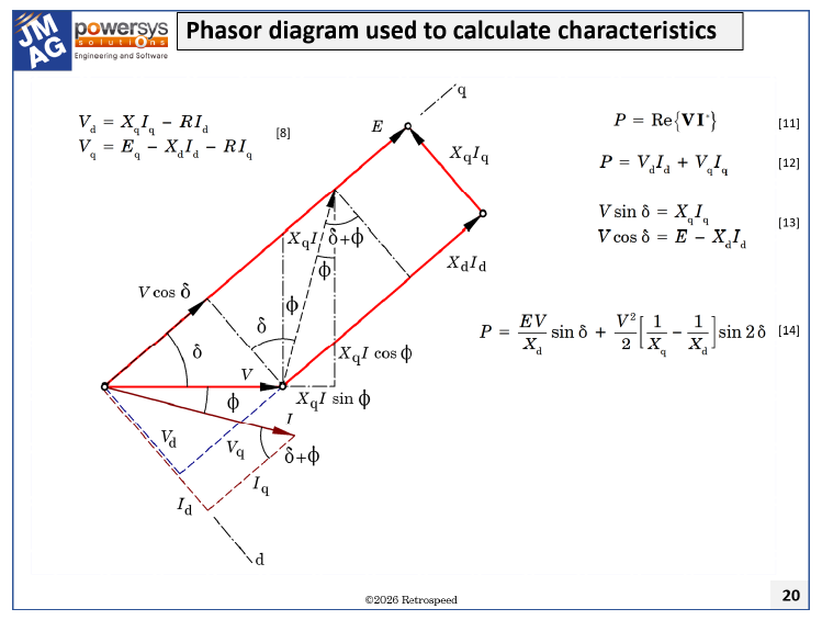
Fig. 2 Classical form of the phasor diagram of a synchronous machine
In classical theory the phasor diagram is often drawn with the terminal voltage V as reference phasor. (See Engineer’s Diary No. 91). This form of the phasor diagram is really just a re-orientation of Fig. 1. Fig. 1 is better adapted for use with inverter-fed machines where the d– and q-axis components are related to their space-vector equivalents in the steady state. But Fig. 2 is better suited when the terminal voltage V is treated as the reference phasor along the real axis. Another related version uses the current I as the reference phasor along the real axis. In both these cases, it is common to do all the analysis using geometric construction and trigonometry, with only limited reference to dq axes.
While Fig. 2 is a voltage phasor diagram, there is also a current phasor diagram derived essentially from the voltage phasor diagram by dividing all the voltages by Xd and adding some additional construction lines, [3]. The current phasor diagram is less common, and it may not always be clear as to whether it is really just a re-scaled voltage diagram or an embodiment of the MMF part of the Potier diagram (see Engineer’s Diary No. 90). The MMF part of the Potier diagram may be a vector triangle of DC-valued field currents, which is arguably confusing to the modern engineer (especially an engineer who relies on direct simulation rather than the ‘cerebral’ abstract methods of our forebears). (See [4]).
A few dashed or chain-dotted construction lines have been added to Fig. 2 to facilitate the algebra. (See Videos 70-72). These construction lines are helpful in defining the main angles, especially the power-factor angle Φ and the load angle δ, which crop up in several locations to help with the trigonometry. One of the most important characteristics to be developed from this diagram is the power / angle relationship (eqn (14) in Fig. 2), but several others are described in Engineer’s Diary No. 91 and in Videos 70-72.
It might seem that this Engineer’s Diary is a somewhat academic commentary on the phasor diagram and its relationship with finite-element calculations. It is also somewhat specialized, and it is recognized that there is a wide variety of conventions in the usage of both phasor diagrams and finite-element methods. Therefore instead of trying to press too hard to establish standard rules or conventions, it is perhaps sufficient to emphasize the importance of mathematical rigour in whatever methods are used to associate them.
Notes
1. The flux-plot was historically the first result obtained from finite-element analysis. From memory, I think line integrals of vector potential came later: although the theory was known, it took time for commercially available finite-element software to develop this as a native facility.
2. Terminal quantities are sometimes called ‘lumped’ parameters. Lumped parameters appear in equivalent circuits, which cannot display distributed quantities. The distributed quantities are more real; the lumped parameters are more virtual. That is why the equivalent circut is a virtual circuit, not a real physical circuit. A wiring diagram is closer to reality than an equivalent circuit, but it does not represent live parameters (voltages, currents, etc) in a form suitable for calculation.
3. This is equally true for voltages induced by rotation and by time-variation of current.
4. Maybe we should call it a ‘stuck flux-plot’.
5. In this regard a phasor differs from a space-vector, which is not restricted as to the time-variation of the corresponding current, voltage, or flux-linkage. In practice, it is common to take the RMS value of voltages, currents, etc. measured by true-RMS-reading instruments, and treat them as phasors, neglecting to extract the fundamental harmonic component. When the quantities involved are reasonably sinusoidal, this does not cause too much trouble, but it would be risky to do this with power-electronic systems (including motor drives), in which many waveforms are not sinusoidal and ‘space-vectors rule’.