Explanation: Model-based Development
This series discusses JMAG's contributions to model-based development. Issue 1 talks about the motivation behind developing "JMAG-RT" for control simulations, which have become a typical solution in model based development. In issue 2, I explained how we are approaching the model based development that we have in mind for JMAG by presenting the new functions involved with JMAG's model base, which was released last summer. Finally, in issue 3, I confirmed that multiphysics is also a solution for model based development and showed that improving the ability to share and distribute information is a necessary condition for CAE to participate in model based development.
This series has examined explanations of conventional model bases while also delving into what exactly model-based development is and what CAE technicians' tasks are. While at first I believed that I had a good understanding of MBD, over the course of this series I soon came to realize that I have much to learn. Though this means that I may have inconvenienced my readers, it provided me with a good chance to rethink model-based development. To finish this series, I would like to study model-based development by focusing on the keywords "zoom-in/zoom-out" and "circulation."
The model's role in a V-model development cycle V-model development cycle
People often pattern their development process after the V-model, using it when explaining model based development, in particular. It conveniently links each step of the development process ("Specification and requirement", "System design", "Subsystem design", "Part design ", "Prototype creation", "Unit evaluation", "Combined evaluation", "System evaluation", and "Comprehensive evaluation") in a workflow, expressing it in an easily understood manner by presenting the study and evaluation progress in a V shape.
The V-model starts with the part specifications and gets more and more detailed as the process moves along. First the prototype becomes more concrete as its trial parts and software become clearer, then it approaches completion thanks to evaluations and revisions, and finally the product comes to fruition when the scope of the evaluations broadens (fig.1).
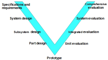 Fig. 1 V-model development workflow
Divergence and convergence
Recently, however, I have begun to feel uncomfortable about this V-model development cycle. After giving it much thought, I have finally reached a conclusion as to the cause of this discomfort, and therefore would like to give a brief explanation. To put it simply, this V-model development cycle is drawn as a single line, while an actual system is composed of multiple subsystems, and each subsystem is an assemblage of a number of components, sub-assemblies, software, and controllers. The configuration starts from the system design and ends with the complete product, but it is not a single line. Instead, it begins to diverge from the first step, splitting into its greatest number of branches when creating a prototype, and beginning to converge up the ladder when evaluations start. I had thought that the old method was strange because no one had ever explained this to me (figures 2 and 3).
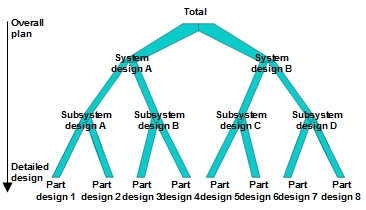 Fig. 2 Divergent development cycle
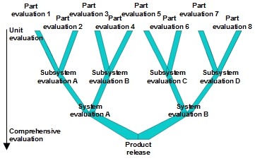 Fig. 3 Convergent development cycle
An image of the actual development cycle
A development cycle, therefore, is a V-model when seen from the front, but when viewed from the side it actually has a large number of branches, like a person's blood vessels. These branches join together again, becoming a completed product in the end. This clarifies the development cycle, and it seems like an obvious conclusion once a person realizes it. This concept is very common in understanding causes and structures of phenomena, and is similar to FTA (Fault Tree Analysis), which is used when analyzing malfunctions (fig.4).
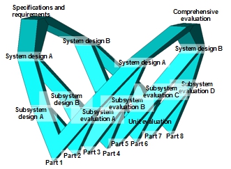 Fig.4 It is possible to image a development cycle in a three-dimensional view
The information necessary for judgment differs from one process to the next
Designers and engineers have to make correct judgments in each development process. In order to do so, however, they need to have the right amount of information. If they have too little information, they cannot make a judgment to begin with, but on the other hand, they may become confused with too much information and accidentally make a wrong decision. Therefore, it is necessary to filter the information at each step along the way: Designers and engineers need to have a broad point of view in the early stages, while in the later stages they have to take a perspective that is closer to the target because the study becomes more detailed.
In the end, the data in this development cycle becomes the model itself. For this reason, one has to be able to zoom in and zoom out on the model, accessing various groups of data freely. Think about it this way: Local data like the magnetic flux density distribution of each part is unnecessary when a person wants a rough estimate of a motor's thermal rating during operation, whereas the level of loss generation during operation becomes vital.
In times like this, one does not need local losses, but when the evaluation target becomes the local demagnetization of the magnet, detailed part geometry and magnetic flux flow are indispensible. This is why people expect the ability to expand and contract the amount of data that they handle for their models freely, depending on the situation. However, data also must be shared between divergent steps in the process, as mentioned above. For example, when two subsystems that are different, like those of an actuator and a controller,have to coordinate and work together, they have to evaluate performance based on data that they have in common.
Fig. 5 gives a clearer perspective of the development process in 3D by adding axes to the image in fig. 4. By looking at it, one can get a better idea of the characteristics required of a model used in model based development: The vertical axis measures the model's level of detail, the horizontal axis measures the level of development, and the longitudinal axis measures the development progress situation (fig. 5). Increasing the speed of the v-model development cycle leads to increases in the speed and efficiency of development itself, so the model needs mobility along the vertical and horizontal axes in addition to a high level of data circulation.
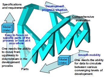 Fig. 5 Exchanging information freely is required for a model
No single step can be skipped or shortcut during development
All of the steps in the process have to be fulfilled in order to get all of the way from start to finish. This fact becomes evident when looking at the v-model because it takes the divergent steps into consideration. Regardless of whether one is working with a prototype or a 3D analysis, the necessary judgments are unavoidable. When all of the risks in a process are not removed at an early stage, they remain in the following steps and lead to problems and setbacks later on. It is impossible to bring the project to fruition if one jumps from one step to the next without passing each detailed design phase (fig. 6).
3D analysis that uses the finite element method (FEM) does the best job of producing results in a detailed design process. If the model is also created following the concept of model based design, one can easily use it in other branches or processes, and improve development speed by doing so.
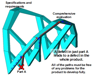 Fig. 6 All the path must be free from any problems
An analysis tool that is conscious of magnification/demagnification and sharing data
Up to this point we have examined the model's role in V-model development. The data that flows through the development process is as universally important as ever, and the concept of model based development has come to be used as a means of raising its versatility and ability to circulate. I stated earlier that people want the ability to freely zoom in on and zoom out of the model itself, but the analysis tools that create and evaluate said model need to be used differently according to the development situation.
A 1D analysis tool
The system's suitability and requirements are studied in the initial stages of development. When preparing to study the exact geometry, one moves forward with logical judgments as to what the system should accomplish, what to get rid of, and what role the various members of construction (subsystems) will play. At this point in time it is best to ignore the physical completion and determine how the model should look. The tool that is typically used in this situation is called a 1D simulator. The model does not have part geometry or material properties, but the performance, functions, I/O relationships, and logic are all defined. MATLAB/Simulink, manufactured by MathWorks, Inc., and AMESim, manufactured by LMS International, are both typical analysis tools.
This is the point where the tasks and roles of the subsystems that make up the system are determined. Control and electric circuits attach importance to logical behavior instead of geometric entities, so they are handled in 1D. At this point in the model's development, it is important to decide what is going to be input and what is going to be output, so an evaluation environment for a model that behaves logically necessary.
A 3D analysis tool
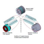
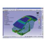
Concrete design studies are carried out in the middle stages of development. Here, one evaluates whether various factors that have been determined upstream (physical validity, completion of the geometry, and how easy it will be to produce) have been fulfilled. The model at this point needs to account for actual geometry and physical properties. Physical simulations that use the finite element method are really unrivaled for these kinds of tasks. When using electromagnetic field analysis, JMAG is the best tool available. With JMAG, one can use a model to evaluate all of the physical systems required by an actual machine. For this reason, a coupled analysis function called multiphysics is necessary as well.
Easy interchange between 1D analysis and 3D analysis
As mentioned earlier, necessary information for judgment differs from one stage to the next. For this reason, one needs the ability to circulate data between the larger and more detailed structures of the development process when using a model in model based design. Instead of displaying everything at once, one has to be able to zoom in on specific parts and zoom out to see the entire picture. Of course, one also has to be able to zoom in and zoom out without much trouble.
JMAG's functions
JMAG provides models that give the ability to expand, contract, and share various amounts of data to meet the requirements of model-based development. I have listed some below.
Supporting 1D analysis
The typical solution for 1D analysis is JMAG-RT, which I introduced issue 1. One can use it to create a motor model with JMAG's highly accurate and high-speed magnetic field analysis. The model uses a voltage signal as its input item, and the analysis obtains the linkage flux, inductance, torque, and phase current value. It provides useful motor data for power electric circuit designs and control designs. We are continuing to develop and improve the JMAG-RT model itself with the aim of raising its universality so that it can be used with C programs, in addition to general control simulators like Simulink.
One can also handle JMAG itself as a 1D model by using its direct link function. In this case it is possible to connect with phenomena for all electrical equipment, not just motors, so the ability to share increases greatly.
Supporting 3D analysis
In 3D analysis, which includes 2D analysis, a model is used that incorporates model geometry and material properties, in addition to following the laws of physics. This is JMAG's area of expertise, as it can run highly accurate electromagnetic field analyses. In addition to solving electromagnetic forces, induction losses, and nonlinear magnetization properties caused by electromagnetic phenomena, it shares all of the information with an analysis simulator. This improves multiphysics support and improves the ability to share data with Abaqus and LMS Virtual.Lab. We are preparing functions that make easy to use magnetic field analysis results with structural analysis and vibration/noise analysis.
In addition to functions that create its own geometry, JMAG-Designer also has a lot of functions that link with CAD. This is made possible with a function that allows CAD and JMAG-Designer to share geometry information files. Changes in CAD geometry are immediately applied in JMAG-Designer, so it is possible to proceed with electromagnetic evaluations of geometry and arrangement designs in parallel. This does not mean that one can share analysis results like multiphysics, but geometry and arrangement designs are extremely important in design development, so the ability to share geometry information will greatly contribute to model based development.
In closing
I originally began this series with the intention of introducing functions in JMAG-Designer that can support model based development. However, as I progressed with my explanation of how JMAG is contributing to model based development, I came to the realization that I had not properly understood model based development itself. After this I began to deviate from introductions of JMAG-Designer's functions and put my efforts into reviewing the model based development process.
This series renewed my understanding of model based design, showing me that it changes the development procedures in a big way. It replaces development data that was previously distributed as documents, layouts, and prototypes into a model, and by doing so raises the ability to share and distribute data. To put another way, it gives designers and engineers the ability to see layouts and specification sheets as models.
I will leave JMAG-Designer's detailed functions to another article. When you read about them, think about how they can raise the level of development information being distributed in your own development cycles. By doing this, you will be able to contribute to streamlining your development process in ways that you had not noticed until now.
(Yoshiyuki Sakashita)
[JMAG Newsletter Winter, 2011]