[W-MA-228] Iron Loss Modeling Techniques: From Measured Data Models to Physical Models

Contents
1. Introduction
2. Loss Components and Modeling Techniques
　2.1 Classification of Iron Loss Components
　2.2 Methods Using Measured Iron Loss Curves
　2.3 Methods Using Mathematical and Physical Models
　2.4 Play Model for Hysteresis Loss Calculation
　2.5 1D Method for Classical Eddy Current Loss Calculation
　2.6 Model Identification for excess loss
3. Consideration of Actual Driving States and Building Factors
　3.1 Inverter Harmonic Iron Loss
　3.2 Building Factors (Stress, Punching Strain)
4. Measurement Comparison Examples for Electric Machines
　4.1 Permanent Magnet Synchronous Motor
　4.2 Switched Reluctance Motor
　4.3 Traction Motor (Permanent Magnet Synchronous Motor)
5. Summary
6. Reference

1. Introduction

In electrical machines, particularly high-power-density and high-speed rotating machines, the physical behavior inside electrical steel sheets has become extremely complex due to the superposition of high-frequency carrier harmonics accompanied by inverter drives and DC bias with magnetic saturation. Since these conditions differ from traditional measurement conditions based on iron loss curves (AC sine waves), they cause discrepancies between measured and analyzed results, making the improvement of prediction accuracy a challenge in design practice. While traditional data-reference methods such as measured iron loss curves and loss maps offer high convenience in operating regions where magnetic flux density varies sinusoidally, they face accuracy limitations in high-frequency and actual driving regions where strong skin effects and local saturation occur.
This white paper reviews modeling techniques for iron loss analysis, focusing on both material properties and actual operating conditions. As an approach to solving these challenges under actual operation, there is a method of separating iron loss into its components. First, we explain the advantages of mathematical and physical model approaches using the "Play Model" for hysteresis loss calculation and the "1D Method" for classical eddy current loss calculation. Next, we describe in detail the parameter identification techniques for excess loss, which must be considered in high-frequency ranges. Finally, we introduce case studies applying these modeling techniques to actual motors (Permanent Magnet Synchronous Motors and Switched Reluctance Motors).

2. Loss Components and Modeling Techniques

2.1 Classification of Iron Loss Components

As shown in Fig. 1, iron loss is classified into hysteresis loss and eddy current loss. Eddy current loss can also be classified into classical eddy current loss caused by the macroscopic electrical resistance of the material and excess loss, which is local eddy current loss associated with domain wall motion. Because these iron loss components are generated by time variations of magnetic flux density inside the steel sheet, accurate evaluation of their behavior requires close attention not only to material properties but also to driving conditions (excitation waveform and frequency).
These components constituting iron loss vary strongly depending not only on the material properties of the steel sheet but also on the time waveform of the magnetic flux density during actual driving (distortion from sine waves, frequency, presence of DC bias, etc.). Therefore, to accurately predict iron loss in actual operating states, appropriate analytical modeling techniques must be selected according to target operating conditions, required computational accuracy, and types of available material data.
Starting from the next section, we will sequentially explain the characteristics and challenges of "Methods Using Measured Iron Loss Curves (Section 2.2)," which have been widely used in practice, and "Methods Using Mathematical Models (Section 2.3 onwards)," which are used to address recent trends toward higher frequencies and power densities.

2.2 Methods Using Measured Iron Loss Curves

In conventional methods used for iron loss calculation, iron loss of steel sheets is measured for each magnetic flux density and frequency. The measured data is used in analysis as a database (iron loss curves). In analysis, time waveforms of magnetic flux density obtained by FEA undergo post-processing such as FFT, and iron loss is predicted by referencing the measured iron loss curves (Fig. 2). Hysteresis loss and eddy current loss are separated as shown in Fig. 3. The advantage of this method is that iron loss curves are provided by material manufacturers and are easy to use. Furthermore, because measured data is used directly, accuracy is high when analysis is performed under conditions close to measurement conditions.
On the other hand, one limitation of this method is that because iron loss is measured with AC, it assumes magnetic flux density varies sinusoidally with time. In other words, errors occur when magnetic flux density waveforms are distorted by DC bias or magnetic saturation. For example, loss in minor loops varies with DC bias components even for the same flux density amplitude, but as long as AC-measured iron loss characteristics are used, the calculated loss remains the same value (Fig. 4). Another limitation is that extrapolation is required in frequency ranges higher than measured frequencies. Extrapolation assumes loss is proportional to the square of frequency, but in reality, it does not increase with the square of frequency due to skin effects. Consequently, extrapolation overestimates eddy current loss (Fig. 5).

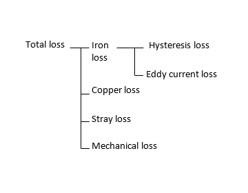
Fig. 1 Classification of loss components

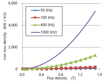
Fig. 2 Iron loss curve (50A1300)

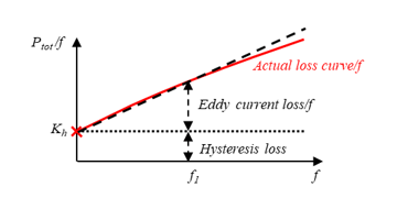Fig. 3 Loss separation with two frequency method
The vertical axis represents loss divided by frequency. The hysteresis loss coefficient Kh can be determined from the y-intercept of the Actual loss curve/f. Subtracting this from the total loss Ptot yields the classical eddy current loss.

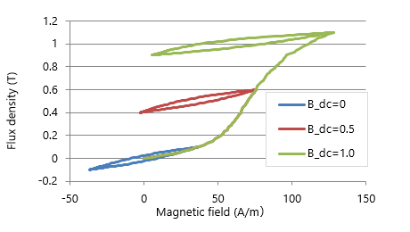Fig. 4 Minor loop losses with different DC components
The three minor loops have the same range of variation in magnetic flux density. However, the width of the magnetic field differs due to the DC component. Since the iron loss curve is measured using AC, it cannot reproduce this difference.

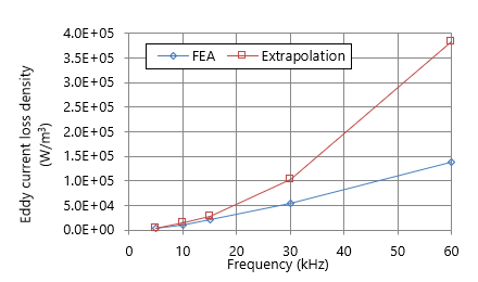Fig. 5 Overestimation of eddy current loss due to the frequency extrapolation (35A210)
The eddy current losses in the iron loss curve, measured up to 10 kHz, were extrapolated by squaring the frequency. Compared to FEA, which can account for the skin effect, the extrapolated results overestimate the losses.

2.3 Methods Using Mathematical and Physical Models

Methods using measured data reproduce actual machines under conditions close to measurement conditions, but magnetic flux density inside actual machines during driving contains not only sine waves but also DC bias components and harmonic components beyond measurement ranges. To further improve loss accuracy, it is necessary to reproduce iron loss caused by arbitrary waveforms of magnetic flux density, introducing new models here: the Play Model for hysteresis loss calculation and the 1D Method for classical eddy current loss calculation.