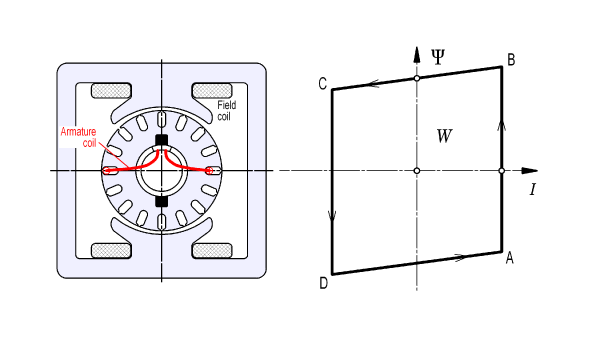
Fig. 1 DC motor and energy-conversion diagram for one coil
The unified theory of electric machines (also known as the generalized theory) flourished in the 20th century at the hands of theorists who sought to deepen their understanding of machine behaviour. Although it would be seen by many as academic, it did provide insights that were (and still are) helpful in linking the behaviour of different machine types into a coherent theoretical framework [3-5]. It also helped with the theory of reference-frame transformations such as Park’s transformation and others, and it provided a deeper understanding of certain particular processes such as commutation in DC machines [3].
However, the unified theory was never central to the process of designing machines. Design methods were (and still are) usually specialized to one type of machine, with technical terms and graphical methods peculiar to that type, often incorporating empirical data and coefficients, and with no obvious connection to the mathematical language of the unified theory; [6-11]. To be fair, some of the theoretical authors did lay out methods that were intended to help the design process, but largely through calculation and simulation of machine behaviour after the machine had been designed.
It can be argued that the unified theory is unnecessary with modern numerical analysis, which is already unified in the sense that it can analyse any machine simply by solving the field equations subject to boundary conditions in time and space. In principle, the designer who is skilled in using these tools does not need to resort to classical formulas (many of which are approximate), and still less to the mathematics of the unified theory.
There are certain fundamental principles (such as Faraday’s law, Ampère’s law, etc.) that are built into numerical analysis tools in electromagnetics, and there are equivalents in other disciplines such as stress analysis and heat transfer. These principles apply in all machines, and in some cases they are obvious because they come to the surface, for example, in calculating a generated EMF waveform which can be expressed as a sequence of samples over one cycle. The samples are instantaneous values that come naturally from a series of finite-element solutions. In a similar way, the average torque can be obtained from a sequence of samples of instantaneous torque (the torque waveform), calculated using the Maxwell stress tensor or an equivalent method.
In the classical theory of machine design and performance, average and RMS values are prominent, and they are often formulated for direct calculation. In contrast, in numerical analysis they have to be obtained from time-integrals or sums of series. In order to formulate average and RMS values of important parameters for direct calculation, the classical methods have to make a priori assumptions about waveforms — most commonly, pure DC or sinusoidal AC. In numerical analysis, such assumptions are not necessary as an inherent part of the analysis, because the solutions are general and do not need simplifying assumptions about waveforms (although much of the analysis is still based on standard waveforms).
This rather lengthy preamble sets the scene for the following proposition: The energy-conversion diagram or flux-MMF diagram can be seen as a unified theory of average torque production, applicable to all machines, requiring almost no mathematical development, and completely compatible with the finite-element method. 1
This assertion is not revolutionary, not new, and may not even be particularly important. It is offered here for no reason other than that it may be interesting. Engineer’s Diary is, after all, a diary, not a textbook.
To illustrate the essential principle of the energy-conversion diagram, it is applied in Video 77 to derive the EMF and torque equations of the DC commutator motor, [11]. Although the DC motor is old, this derivation is not known to have been presented before. We might ask, why do we need a derivation of these equations by a different method? The answer is that while we may not have an absolute need for a new derivation, the method avoids the BLV and BLI formulas which are used by almost all traditional textbooks and which are (i) difficult to justify rigorously and (ii) unsuitable for calculation by the finite-element method. In other words, what we have is a derivation of the EMF and torque equations that is (a) completely rigorous and (b) suitable for calculation and verification by the finite-element method.
There’s a third point: the energy-conversion method presented here for the DC machine is directly applicable to any electric machine. That’s because it builds on the conditions for one coil, and every electric machine contains windings that are simply series / parallel connections of coils. The generalization of the method to all electric machines — from a single coil in a ‘primitive’ machine (in this case the armature of a DC motor) — is close to the teaching of Gabriel Kron in the 1930s [5], while the energy-conversion principle was taught by Herbert C. Roters in the same period [16]; but neither of them could have imagined the advanced numerical analysis tools that we have today. Nor could either of them have foreseen that numerical analysis would finally unify the theory of electric machines, with the energy-conversion loop at the heart of the process for design calculations as well as performance analysis.
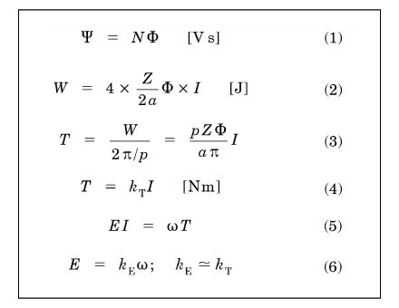
Fig. 2 Equations
Consider a single coil in the armature of a DC motor, terminated at two adjacent commutator segments shorted by the upper brush, Fig. 1. This is where the current I reverses its direction, while the linkage of the coil with the pole-flux Φ produced by the field winding is at its maximum value Ψ, given by eqn. (1) in Fig. 2. N is the number of turns on the coil. The current-reversal takes place very quickly and we can represent it at the upper brush by the line BC in Fig. 1. This line is inclined owing to the flux-linkage LI associated with the coil inductance. After a further rotation through one pole-pitch, the two commutator segments become shorted by the opposite (lower) brush, and the current reverses again, this time along DA; again the transition is very rapid.
The transitions AB and CD are both vertical because the current is constant when the coil is not shorted by a brush. The operation of this one coil can therefore be characterized by the closed rectangular locus ABCD, which is known as the flux-linkage/current loop. It is a well-established result in the theory of electromagnetic energy conversion that the enclosed area W = ABCD represents energy converted from electrical to mechanical or vice-versa during one cycle of operation. This implies that there must be torque. Neglecting losses, and relying on the conservation of energy, the average torque over one cycle must be W/(2π/p) where 2π/p is the angle of rotation over one cycle and p is the No. of pole-pairs (p = 1 here).
If Z is the total No. of conductors in the armature, (i.e., twice the total No. of turns), and each conductor is carrying the current I/a (where a is the No. of parallel paths in the winding), then from the diagram and eqn. (1) we can write eqn. (2). The average electromagnetic torque is thus given by eqn. (3), which can be written as eqn. (4).
kT is the torque constant, i.e., the average torque per ampere. Eqn. (4) is recognized as a common standard torque formula widely quoted and used especially with servomotors and in simpler forms of motor control.
Commutator action leaves a residual torque ripple at the commutator-segment passing frequency, which defines ‘one electrical cycle’ of the energy-conversion loop.
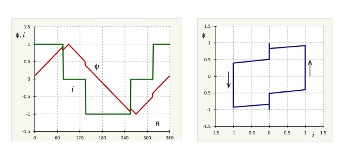
Fig. 3 Current and flux-linkage waveforms; brushless DC motor
Again neglecting losses, energy conservation requires eqn. (5), where E is the average generated-EMF or back-EMF and ω is the mechanical angular velocity. From this and eqn. (3) we deduce eqn. (6), which gives the EMF constant kE. E is a DC voltage generated purely by rotation. It has no Ldi/dt component. The constant kE is the generated volts per rad/sec, and according to the ideal theory it is equal to kT; but in practice kE is not exactly equal to kT because of various imperfections in the process; indeed saturation causes kT to decrease at high current, so it is not constant.
We have done enough to show the derivation of the main design equations for the DC motor from the energy-conversion loop, Figs. 1 and 2. Since the energy-conversion loop can be calculated from a sequence of (i, ψ) values over one electrical cycle, the theory is compatible with finite-element computations and it gives average values of torque and EMF over one electrical cycle.
The next step up in complexity from the basic DC commutator motor is the brushless DC motor which has a PM rotor, usually of the surface-magnet type, and a 3-phase stator. It is driven by squarewave currents from an inverter with 2 phases conducting at any time. The current can be regulated by chopping so that it has a waveform close to that shown here. The blocks of phase current are 120° wide, and they are synchronous with the flux-linkage waveform which is approximately triangular, Fig. 3.
When the flux-linkage ψ is plotted vs. the current i, we get a Lissajous figure with two parts, one for the positive half-cycle and one for the negative half-cycle, enclosing a total area W. The phase shift causes one part to be displaced relative to the other part, but as long as the phase shift is limited there is no effect on the loop area or the torque. The main point is the similarity of the flux-linkage / current loop to that of the single coil in the DC commutator motor. The BLDC motor can be regarded as an inside-out DC motor with only a small number of phases, in which the inverter phase-legs perform the function of the commutator in reversing the current twice per cycle in each phase.
The average electromagnetic torque can be calculated from the energy W converted in each of the m phases in each electrical cycle covering 2π/p mechanical radians; thus T = mpW/2π. If this is related to the DC current I at the input to the inverter, we get eqn. (4). This definition of I is necessary because the phase current is alternating with a waveform that is near to a 120° square-wave.
It is commonplace with brushless servomotors to use eqn. (6), but here we should define E as the mean value of the rectified EMF on open-circuit. The reason is that eqns. (4 and 6) imply the pure energy-conversion equation (5). These principles are important for servomotors and they are thoroughly analyzed in [GB 8].
Using the energy-conversion diagram, these formulas evolve quite simply and even elegantly from the DC commutator motor to the brushless DC motor, in spite of the differences in the design and operation of these machines. They can also be applied to almost any electric machine of any type, and detailed examples are developed for the switched reluctance motor and for a class of AC machines (both synchronous and asynchronous) in Videos 77-78. (Video No. 78 is scheduled to be released End of October.)
Notes
1 For a comprehensive treatment of the energy-conversion diagram and its application to different types of machines, see [12-15].
References
[1] Hendershot J.R. and Miller T.J.E., Design of Brushless Permanent-Magnet Machines, Motor Design Books LLC, ISBN 978-0-9840687-0-8, 2010, sales@motordesignbooks.com (Green Book)
[2] Hendershot J.R. and Miller T.J.E., Design Studies in Electric Machines, Motor Design Books LLC, ISBN 978-0-9840687-4-6, 2022, (Blue Book)
[3] Jones C.V., The Unified Theory of Electrical Machines, Butterworths, 1967.
[4] Adkins B., The General Theory of Electrical Machines, Chapman & Hall, 1957.
[5] Kron G., The Application of Tensors to the Analysis of Rotating Electrical Machinery, General Electric Review, 1938.
[6] Alger P.L., Induction Machines, Their Behavior and Uses, Second Edition, Gordon and Breach, New York, 1970.
[7] Veinott C.G., Theory and design of small induction motors, McGraw-Hill, 1959.
[8] Kostenko M. and Piotrovsky L., Electric Machines, MIR Publishers, 1974.
[9] Walker J.H., Operating Characteristics of Salient-Pole Machines, Proc. I.E.E. - Part II: Power Engineering, 100 (73), 1953, pp. 13–24. doi:10.1049/pi 2.1953.0004 and J.I.E.E., Vol. 112, No. 2, 1953. pp. 13–23
[10] Doherty R.E. and Nickle C.A., Synchronous Machines I — An Extension of Blondel’s Two-Reaction Theory, Transactions A.I.E.E., June 1926, 912-947
[11] Clayton A.E and Hancock N.N., The Performance and Design of Direct Current Machines, 3rd edn., Pitman, London, 1959-66
[12] Deodhar R.P., The Flux-MMF Diagram Technique and Its Applications in Analysis and Comparative Evaluation of Electrical Machines, Ph.D. thesis, University of Glasgow, October 1996, https://theses.gla.ac.uk/3241/
[13] Staton D.A., Soong, W.L., Deodhar R.P. and Miller T.J.E., Torque prediction using the flux-MMF diagram in AC, DC and reluctance motors, IEEE Trans. Industry Applications, Vol. 32, No.1, Jan Feb. 1996, pp. 180–188
[14] Deodhar R.P., Staton D.A., Jahns T.M. and Miller T.J.E., Prediction of cogging torque using the flux-MMF diagram technique, IEEE Trans. Industry Applications, Vol. 32, No. 3, May-Jun 1996, pp. 569–576
[15] Deodhar R.P., Staton D.A. and Miller T.J.E., Modelling of skew using the flux-MMF diagram, IEEE Trans. Industry Applications, Vol. 32, No. 6, Nov-Dec 1996, pp.1339-1347
[16] Roters H.C., Electromagnetic Devices, John Wiley & Sons, N.Y., 1941